Excel FILTER Function Explained: Dynamic Data Extraction & Advanced Filtering Techniques

The Excel FILTER Function is a revolutionary tool for extracting data dynamically based on multiple conditions. With dynamic arrays, data extraction, and non-destructive analysis, this function updates results automatically when your source data changes. Whether you’re a beginner or advanced user, this guide covers every aspect—from basic syntax to complex filtering techniques and troubleshooting—to help you master Excel’s filtering power.

What is Excel FILTER Function

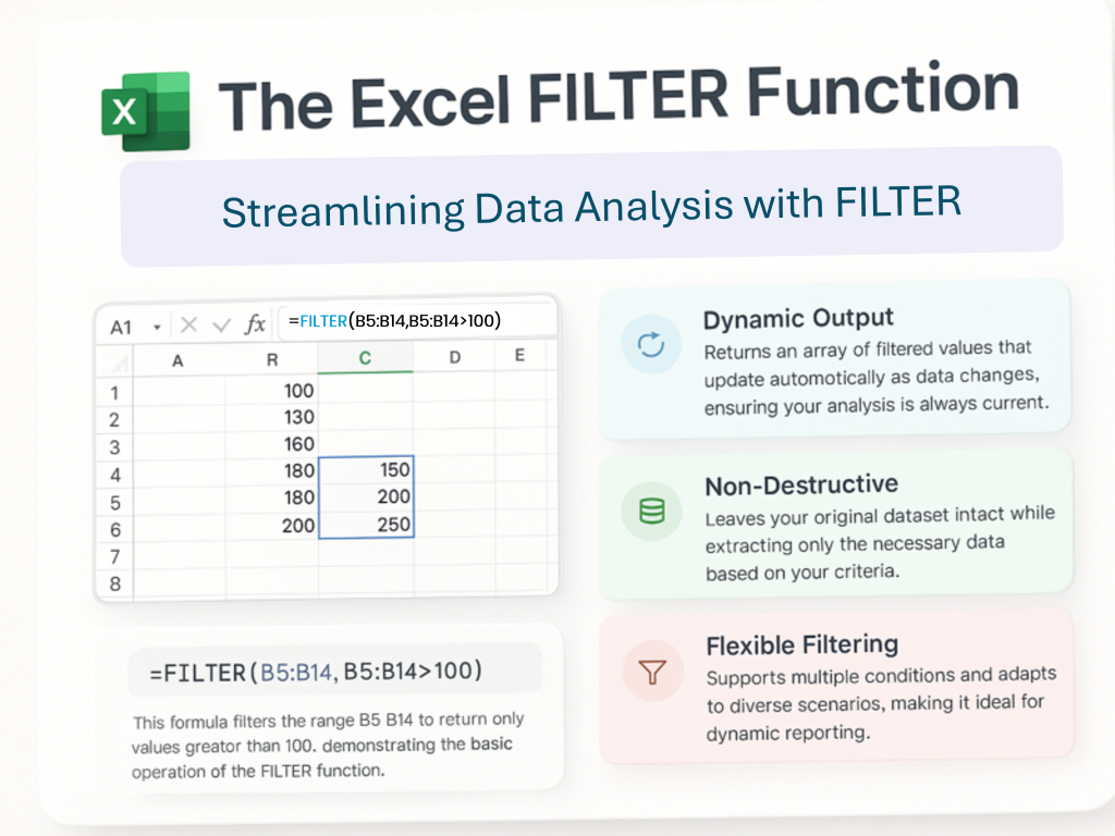
The FILTER function extracts matching values from a dataset without altering the original data, updating results dynamically as conditions change. It is newly added function in the Excel,  perfect for isolating, analyzing, and inspecting data in real time.

• Dynamic Output:: Returns a Dynamic arrays of filtered values that update automatically as data changes, ensuring your analysis is always current.
• Non-Destructive:: Leaves your original dataset intact while extracting only the necessary data based on your criteria.
• Flexible Filtering:: Supports multiple conditions and adapts to diverse scenarios, making it ideal for dynamic reporting.

=FILTER(B5:B14, B5:B14>100)

This formula filters the range B5:B14 to return only values greater than 100, demonstrating the basic operation of the FILTER function.

FILTER Function Syntax

The syntax for the FILTER function is simple and powerful. We often search for Excel filter syntax and array filtering to learn how to set up this function properly. Understanding the parameters allows you to control what data is returned and handle cases when no data matches your criteria.

=FILTER(array, include, [if_empty])

• Array:: The range or array to filter, representing the source dataset.
• Include:: A Boolean array representing conditions that must be met for data extraction.
• If_Empty:: An optional parameter that returns a value if no data meets the criteria, preventing errors.

Purpose of the FILTER Function

The purpose of the FILTER function is to quickly sift through large datasets and extract only those records that meet your specified conditions. Popular search terms like filter range and criteria extraction make it clear that this function is all about isolating data without modifying the source. It’s ideal for focused data analysis and reporting.

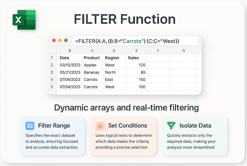
• Filter Range:: Specifies the exact dataset to analyze, ensuring focused and accurate data extraction.
• Set Conditions:: Uses logical tests to determine which data meets the criteria, providing a precise selection.
• Isolate Data:: Quickly extracts only the required data, making your analysis more streamlined.

Return Value of the FILTER Function

The FILTER function returns a dynamic array of values that satisfy your conditions. This output is updated automatically if the source data or criteria change, which is why many search for dynamic result and filtered array when learning about this feature. The function provides consistent and reliable output for real-time analysis.

• Filtered Array:: Produces an array containing only the data that meets your conditions, ensuring clear results.
• Automatic Refresh:: Updates instantly when your dataset or criteria change, keeping your analysis accurate.
• Consistent Output:: Maintains reliable results that can be easily used in further calculations or dashboards.

Using the FILTER Function

Using the FILTER function involves applying logical tests to your dataset to extract the desired information. It is popular among users looking for data extraction, dynamic filtering, and logical tests in Excel. This function evaluates each element of your data range and returns only those that satisfy the conditions set.

• Logical Testing:: Applies conditions that return TRUE or FALSE, ensuring only qualifying data is shown.
• Dynamic Extraction:: Updates the filtered results automatically as data or criteria change.
• Non-Destructive Analysis:: Extracts data without modifying your original dataset, preserving your raw data.

=FILTER(B5:B14, B5:B14>100)

This formula filters B5:B14 for values greater than 100, showcasing a straightforward logical test.

Basic Example of the FILTER Function

A basic example of the FILTER function demonstrates its ease of use for beginners. Users frequently search for basic FILTER example and simple Excel filtering. This example shows how to extract values from a single column based on a numeric condition, forming the foundation of more advanced techniques.

=FILTER(B5:B14, B5:B14>100)

• Simple Condition:: Uses one logical test to determine which values to return.
• Direct Extraction:: Immediately outputs only those values that meet the condition.
• User-Friendly:: Perfect for beginners learning the fundamentals of Excel filtering.

Explanation: The formula returns values from B5:B14 that are greater than 100, illustrating the basic functionality of FILTER.

Filter for “Red” Group Example

Filtering by group allows you to extract records for a specific category, such as “Red.” This technique is popular for conditional filtering and group data extraction. It can be implemented using a cell reference for dynamic criteria or by hardcoding the value directly.

=FILTER(B5:D14, D5:D14=H2, "No results")

• Cell Reference:: Uses a cell (H2) as the criterion for dynamic filtering.
• Hardcoded Value:: Alternatively, directly specify “Red” within the formula for static criteria.
• Group Isolation:: Extracts all rows where the group column matches the specified value.

Explanation: When H2 contains “Red,” this formula returns all matching rows from B5:D14.

Handling No Matching Data

When no data matches your criteria, the FILTER function can return a custom message instead of an error. Searches for no matching data and if_empty argument are common. This feature improves the usability of your reports by clearly indicating when no results are found.

=FILTER(array, include, "No results")

• Custom Message:: Displays a user-friendly message like “No results” if no data meets the criteria.
• Error Prevention:: Avoids #CALC! errors by providing a fallback value.
• Clear Communication:: Helps users understand that no matching data was found without encountering an error.

Explanation: The formula returns “No results” when no matching data is found, maintaining clarity in your output.

Filtering Values Containing Specific Text

Filtering data for specific text is essential when working with strings. This method is popular for text filtering and partial matches. By combining FILTER with SEARCH and ISNUMBER, you can effectively extract rows that contain the desired text.

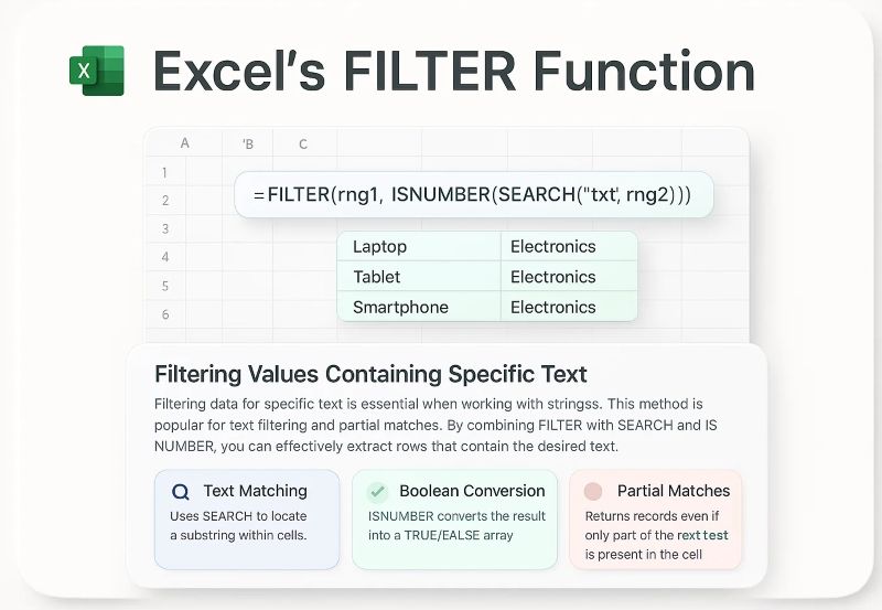
=FILTER(rng1, ISNUMBER(SEARCH("txt", rng2)))

• Text Matching:: Uses SEARCH to locate a substring within cells.
• Boolean Conversion:: ISNUMBER converts the result into a TRUE/FALSE array.
• Partial Matches:: Returns records even if only part of the text is present in the cell.

Explanation: This formula filters rng1 for rows where “txt” is found in rng2, making text-based filtering possible.

Filtering Data by Date

Filtering by date is a powerful way to extract records within specific time frames. It is a top search for filter by date and Excel date filtering. Using functions like MONTH allows you to set criteria based on months, years, or custom date ranges, ensuring your analysis is timely.

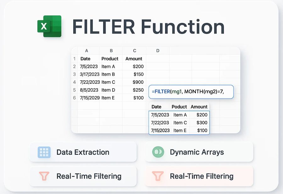
=FILTER(rng1, MONTH(rng2)=7, "No data")

• Date Comparison:: Compares the month of dates to a specific value.
• Time-Sensitive:: Automatically updates as the date changes in the dataset.
• Custom Periods:: Allows you to filter data for any specific period, like a month or year.

Explanation: This formula filters data where the date in rng2 falls in July, ideal for time-based analysis.

Multiple Criteria Filtering

Using multiple criteria in FILTER is essential for complex data extraction. Users search for multiple criteria filtering and AND/OR logic. By combining conditions with multiplication for AND logic or addition for OR logic, you can precisely extract the desired records from your dataset.

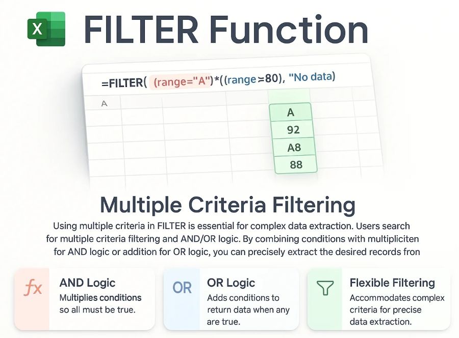
=FILTER(range, (range="A")*(range>80), "No data")

• AND Logic:: Multiplies conditions so all must be true.
• OR Logic:: Adds conditions to return data when any are true.
• Flexible Filtering:: Accommodates complex criteria for precise data extraction.

Explanation: The formula returns records where the value equals “A” and is greater than 80, demonstrating multi-criteria filtering.

Complex Criteria Filtering

For advanced scenarios, complex criteria filtering enables you to build multi-layered conditions. This method is favored by users searching for complex criteria and advanced Excel filtering. By nesting functions and using Boolean logic, you can filter data based on several simultaneous conditions.

=FILTER(data, (LEFT(account,1)="x")*(region="east")*NOT(MONTH(date)=4))

• Nested Functions:: Combines multiple functions to create advanced conditions.
• Multi-Level Testing:: Ensures data meets all specified conditions simultaneously.
• Extended Flexibility:: Adapts to intricate filtering requirements for detailed analysis.

Explanation: This formula extracts records where the account starts with “x,” the region is “east,” and the month is not April.

Using Wildcards with FILTER

Wildcards aren’t directly supported in FILTER, but you can mimic them using SEARCH. Many users look up wildcard filtering and partial match to handle text-based conditions. This method enables flexible text searches even without native wildcard support.

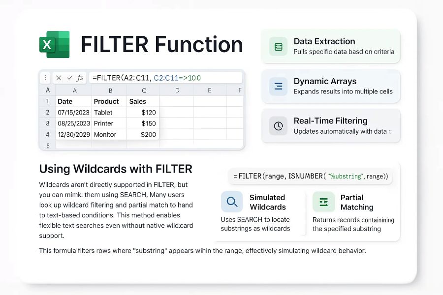
=FILTER(range, ISNUMBER(SEARCH("substring", range)), "No results")

• Simulated Wildcards:: Uses SEARCH to locate substrings as wildcards.
• Partial Matching:: Returns records containing the specified substring.
• Enhanced Flexibility:: Offers a workaround for advanced text filtering needs.

Examples: Wildcards enhance Excel’s FILTER function by enabling pattern-based data extraction, moving beyond exact matches to find relevant information efficiently.

=FILTER(A1:B10, ISNUMBER(SEARCH("apple*", A1:A10)))
=FILTER(A1:B10, ISNUMBER(SEARCH("*.com", B1:B10)))
=FILTER(A1:B10, LEFT(A1:A10, 1)="J")

 

Explanation: Using wildcards with FILTER significantly expands data filtering capabilities, allowing for more flexible and powerful data analysis within Excel.

Nesting Dynamic Array Formulas

Nesting dynamic array formulas, such as combining SORT with FILTER, is a favorite among advanced users searching for nesting dynamic arrays and advanced dynamic formulas. This approach creates elegant and powerful solutions that update automatically.

=SORT(FILTER(A2:C13, B2:B13=F1), 2, 1)

• Layered Functions:: Combines multiple functions to perform sequential operations.
• Enhanced Sorting:: Automatically sorts the filtered results.
• Dynamic Arrays:: Leverages Excel’s dynamic capabilities for fluid data manipulation.

Explanation: Filters data based on F1 and sorts the results by the second column in ascending order.

How to Count Unique Values

Counting unique values in filtered data is simplified by combining UNIQUE and FILTER functions. Users frequently search for count unique values and dynamic arrays. This technique provides an efficient way to tally distinct records that meet specific conditions.

=COUNTA(UNIQUE(FILTER(A2:A20, B2:B20="Yes")))

• Distinct Count:: Isolates unique values from the filtered dataset.
• Conditional Counting:: Counts only entries that satisfy a particular condition.
• Efficient Analysis:: Simplifies data review by focusing on distinct records.

Explanation: Counts unique entries in A2:A20 where B2:B20 equals “Yes.”

FILTER with Boolean Logic and Two Criteria

Using Boolean logic with the FILTER function allows you to combine multiple criteria seamlessly. Many users search for FILTER with Boolean logic and two criteria filtering. This method uses multiplication for AND logic and addition for OR logic, ensuring robust and precise data extraction.

=FILTER(A2:C13, (C2:C13=F2) * ((B2:B13=E2) + (B2:B13=E3)), "No results")

• AND Conditions:: Multiplies Boolean arrays to require all conditions are met.
• OR Conditions:: Adds Boolean arrays to return results if any condition is true.
• Robust Filtering:: Handles multiple overlapping criteria for precise data extraction.

Explanation: Returns records where column C equals F2 and column B is either E2 or E3.

Filtering with Dynamic Dropdown Lists

Dynamic dropdown lists make your dashboards interactive by letting users choose filtering criteria. This feature is often searched as dynamic dropdown filtering and interactive filtering. It updates results in real time based on the user’s selection, creating a personalized data view.

=FILTER(data_range, criteria_range=J2, "No results")

• User Interaction:: Lets users select criteria via a dropdown menu.
• Real-Time Updates:: Instantly refreshes the filtered data based on the dropdown selection.
• Custom Views:: Tailors data display without altering the source dataset.

Explanation: Filters data based on the value selected in cell J2, providing a dynamic and interactive experience.

Filtering Specific Columns

When you need only certain columns from a large dataset, you can extract them using a nested FILTER formula. This approach is popular for filtering specific columns and non-contiguous filtering. It allows you to focus on the most relevant data while omitting unnecessary details.

=FILTER(FILTER(A2:C13, B2:B13=F1), {TRUE, FALSE, TRUE})

• Selective Output:: Returns only the chosen columns from the filtered results.
• Custom Column Extraction:: Filters out unwanted columns for a cleaner view.
• Enhanced Clarity:: Reduces data clutter by displaying only pertinent information.

Explanation: Filters rows based on F1 and then returns only the 1st and 3rd columns from the data.

Limiting the Number of Rows Returned

Sometimes, you need to restrict the number of rows output by your FILTER function, especially in limited workspace scenarios. This technique is popular for limiting rows and INDEX with SEQUENCE. By combining FILTER with INDEX and SEQUENCE, you can control the exact number of rows returned.

=IFERROR(INDEX(FILTER(A2:C13, B2:B13=F1), SEQUENCE(2), SEQUENCE(1, COLUMNS(A2:C13))), "No result")

• Row Limitation:: Restricts the output to a specific number of rows.
• Automated Sequencing:: Uses SEQUENCE to generate dynamic row indices.
• Error Handling:: IFERROR manages cases when there are fewer rows than expected.

Explanation: Returns only the first two rows from the filtered data, ensuring your display area is not overwhelmed.

Aggregation with FILTER (Sum, Average, Min, Max)

Aggregating data with FILTER can be achieved by combining it with functions like SUM, AVERAGE, MIN, and MAX. Searches for aggregate with FILTER and data aggregation are common. This technique allows you to perform calculations on just the filtered subset, streamlining your analysis.

=SUM(FILTER(C2:C13, B2:B13=F1, 0))

• Sum Calculation:: Adds all values from the filtered dataset.
• Average Calculation:: Computes the mean of filtered values.
• Min/Max Analysis:: Determines the smallest or largest value among the filtered data.

Explanation: Sums the values in C2:C13 for rows where column B equals F1, returning 0 if no results are found.

Case-Sensitive FILTER Formula

By default, the FILTER function is case-insensitive. To perform case-sensitive filtering, nest the EXACT function within FILTER. Users often search for case-sensitive filtering and EXACT function in FILTER. This method ensures that only entries matching the exact case are returned.

=FILTER(A2:C13, EXACT(B2:B13, "a"), "No results")

• Exact Matching:: Differentiates between uppercase and lowercase letters.
• Improved Accuracy:: Returns results only when the case matches exactly.
• Specialized Filtering:: Ideal for data where case sensitivity is crucial.

Explanation: Filters rows in A2:C13 where column B exactly matches the lowercase “a,” ensuring precise case-sensitive results.

Filtering Duplicates and Blanks

Filtering duplicates and blanks is essential for data cleanup. This method, often searched as filter duplicates and remove blanks in Excel, uses COUNTIFS with FILTER to return only repeated or complete records, ensuring your dataset remains clean and accurate.

=FILTER(A2:C20, COUNTIFS(A2:A20, A2:A20, B2:B20, B2:B20, C2:C20, C2:C20)>1, "No results")

• Filter Duplicates:: Extracts rows that appear more than once in the dataset.
• Remove Blanks:: Excludes rows with empty cells to maintain data quality.
• Data Cleanup:: Ensures your analysis is based on complete, reliable information.

Explanation: This formula returns duplicate rows from A2:C20 by checking the count of each record across all columns.

FILTER Function Examples

Real-world examples highlight the versatility of the FILTER function. This section includes practical examples that users search for when they need to see FILTER function examples in action, from unique value extraction to data cleanup.

Unique Values Ignoring Blanks

=UNIQUE(FILTER(B5:B16, B5:B16<>""))

Unique Extraction:: Filters out blanks and returns only unique values using the UNIQUE function. Removes blank cells from B5:B16 and outputs a list of unique entries.

Average Call Time per Month

=AVERAGE(FILTER(E2:E13, MONTH(B2:B13)=7, 0))

Aggregated Analysis:: Calculates the average call time for a specific month by filtering data accordingly. Computes the average of call durations in July, returning 0 if no data is available.

Removing Blank Rows

=FILTER(A2:C12, (A2:A12<>"")*(B2:B12<>""), "No results")

Data Cleanup:: Eliminates rows with blank cells to maintain a clean dataset for analysis. Filters out any rows in A2:C12 with blanks in either column A or B.

Extract Common Values from Two Lists

=FILTER(B5:B16, COUNTIF(D5:D14, B5:B16)>0, "No results")

Common Data:: Extracts values found in both lists, highlighting overlapping information. Returns values from B5:B16 that are also present in D5:D14.

Download Example File

Boost your Excel skills with our free Excel example file featuring sample data, dynamic arrays, and 20 practical Excel filter examples. This downloadable file includes two comprehensive tables—Sales Data and Employee Data—plus formulas that showcase real-world filtering techniques. Whether you’re a beginner or advanced user, this sample file is designed to help you understand and apply dynamic filtering in Excel effortlessly.

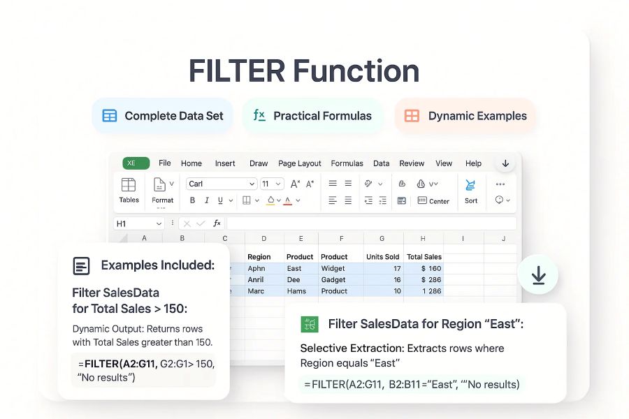
• Complete Data Set: Contains two detailed tables with sample data, ideal for practicing various filtering scenarios.
• Practical Formulas: Includes 20 ready-to-use FILTER formulas, demonstrating basic to advanced filtering techniques.
• Dynamic Examples: Showcases dynamic array capabilities in Excel, enabling you to see real-time data updates.
• User-Friendly Format: Easy to open, copy, and paste into your own Excel workbook for immediate hands-on practice.

Excel FILTER Function Examples

Examples Included:

1. Filter SalesData for Total Sales > 150:
   Dynamic Output: Returns rows with Total Sales greater than 150.

   =FILTER(A2:G11, G2:G11>150, "No results")

2. Filter SalesData for Region “East”:
   Selective Extraction: Extracts rows where Region equals “East”.

   =FILTER(A2:G11, B2:B11="East", "No results")

3. Filter SalesData for Product “Widget”:
   Product Focus: Returns rows with Product “Widget”.

   =FILTER(A2:G11, D2:D11="Widget", "No results")

4. Filter SalesData for Units Sold ≥ 10:
   Quantity Filter: Extracts rows with at least 10 units sold.

   =FILTER(A2:G11, E2:E11>=10, "No results")

5. Filter SalesData for Date ≥ 1/10/2023:
   Time-Based Filtering: Returns sales records on or after January 10, 2023.

   =FILTER(A2:G11, A2:A11>=DATE(2023,1,10), "No results")

6. Filter SalesData for Region “East” AND Product “Gadget”:
   Combined Conditions: Retrieves rows meeting both criteria.

   =FILTER(A2:G11, (B2:B11="East")*(D2:D11="Gadget"), "No results")

7. Filter SalesData with IF_EMPTY (Total Sales > 500):
   Fallback Message: Returns “No results” if no rows exceed 500 in Total Sales.

   =FILTER(A2:G11, G2:G11>500, "No results")

8. Filter EmployeeData for Department “Sales”:
   Department Focus: Extracts employee records from the Sales department.

   =FILTER(A14:G21, C14:C21="Sales", "No results")

9. Filter EmployeeData for Salary > 55000:
   Salary Filter: Returns rows with Salary greater than 55,000.

   =FILTER(A14:G21, E14:E21>55000, "No results")

10. Filter EmployeeData for Bonus > 5000:
    Bonus Condition: Extracts employees with Bonus greater than 5,000.

    =FILTER(A14:G21, F14:F21>5000, "No results")

11. Filter EmployeeData for Hire Date ≥ 1/1/2018:
    Date Filter: Retrieves employees hired on or after January 1, 2018.

    =FILTER(A14:G21, D14:D21>=DATE(2018,1,1), "No results")

12. Filter EmployeeData for Department “IT” AND Salary > 60000:
    Combined Criteria: Returns IT employees earning more than 60,000.

    =FILTER(A14:G21, (C14:C21="IT")*(E14:E21>60000), "No results")

13. Filter SalesData with OR: Region “East” OR “North”:
    Flexible Filtering: Returns rows where Region is either “East” or “North”.

    =FILTER(A2:G11, (B2:B11="East")+(B2:B11="North"), "No results")

14. Filter SalesData for Region “West” AND Units Sold ≥ 10:
    Strict Criteria: Retrieves rows from West with at least 10 units sold.

    =FILTER(A2:G11, (B2:B11="West")*(E2:E11>=10), "No results")

15. Filter SalesData for Salesperson containing “an”:
    Partial Match: Extracts rows where the Salesperson name includes “an” (e.g., Anna, Jane).

    =FILTER(A2:G11, ISNUMBER(SEARCH("an", C2:C11)), "No results")

16. Filter EmployeeData for Name containing “John”:
    Text Search: Returns records with “John” in the Name field.

    =FILTER(A14:G21, ISNUMBER(SEARCH("John", B14:B21)), "No results")

17. Return Specific Columns from SalesData (Date, Salesperson, Total Sales):
    Selective Columns: Displays only columns A, C, and G.

    =FILTER(FILTER(A2:G11, A2:A11<>""), {TRUE, FALSE, TRUE, FALSE, FALSE, FALSE, TRUE})

18. Return Specific Columns from EmployeeData (Name and Total Compensation):
    Focused View: Shows only the Name and Total Compensation columns.

    =FILTER(FILTER(A14:G21, A14:A21<>""), {FALSE, TRUE, FALSE, FALSE, FALSE, FALSE, TRUE})

19. Count Rows in SalesData with Total Sales > 150:
    Row Counting: Provides a tally of rows meeting the condition.

    =COUNTA(FILTER(A2:G11, G2:G11>150, ""))

20. Sum Total Sales for Region “West” in SalesData:
    Aggregated Sum: Calculates the total sales amount for West region.

    =SUM(FILTER(G2:G11, B2:B11="West", 0))

Common Errors with the FILTER Function

Common errors such as #NAME, #REF, and others can occur when using the FILTER function. This information is crucial for troubleshooting, especially for users searching for common FILTER errors and error resolution in Excel. Understanding these errors helps you resolve them quickly and maintain robust formulas.

• #NAME Error:: Occurs if FILTER is used in an unsupported Excel version.
• #REF Error:: Happens when the formula references closed workbooks.
• Error Handling:: Wrap your formulas in IFERROR to manage unexpected issues.

Recognize and resolve these common errors by checking your function usage and ensuring compatibility with Excel 365 or Excel 2021.

FILTER Function Usage Notes and Troubleshooting

Understanding common pitfalls and troubleshooting techniques is vital when working with the FILTER function. This topic is widely searched under FILTER errors and usage notes. By adhering to these guidelines, you can prevent errors like #SPILL, #CALC, and dimension mismatches, ensuring smooth performance.

• Spill Behavior:: Ensure adjacent cells are clear so that the dynamic array can spill correctly.
• Array Compatibility:: Verify that the dimensions of the array and criteria match perfectly.
• Error Management:: Use IFERROR to gracefully handle unexpected issues in your formula.

Conclusion and Final Thoughts

The Excel FILTER function is an indispensable tool for anyone serious about data analysis. It allows you to extract, manipulate, and analyze data dynamically, with results that update automatically as conditions change. With this guide, covering everything from basic syntax and examples to advanced filtering, troubleshooting, and dynamic reporting, you now have all the tools you need to master Excel’s powerful filtering capabilities.

• Comprehensive Learning:: Covers topics from basic usage to advanced techniques for dynamic filtering.
• Dynamic Capabilities:: Automatically refreshes results to reflect real-time data changes.
• Practical Applications:: Equips you with techniques to solve real-world data challenges effectively.

This guide has provided a thorough overview of the Excel FILTER function, empowering you to enhance your data analysis and reporting skills with dynamic, flexible filtering. Please share your feedback, and let us know if you need any specific formula to Filter the data in the comments section below.