Excel Formula If Cell Contains Text Then Return Value in Another Cell

Here is the Excel Formula If Cell Contains Text Then to Return Value in Another Cell. This is the very useful formula when we deal with strings. We can check if a cell contains a string value and write something in another cell or adjacent column. The following examples shows you the different scenarios with formulas to create strings in a new column based on the data in another column.

In this topic:

• Excel Formula to Check a Cell and Return Value in Another Cell
• Tracing of Excel Formula Calculation Steps
• Clear Explanation of Formula for Matching and Returning Values
• Free Excel File to Download and Check the Examples

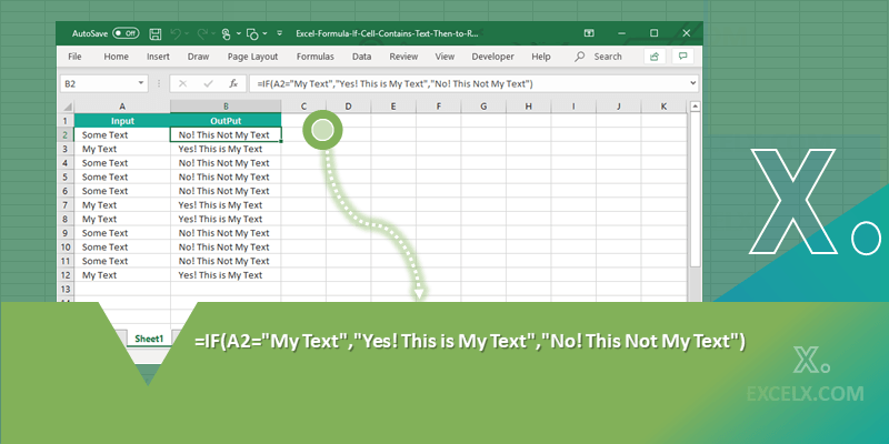
Excel Formula to Check If a Cell Contains Text Then Return Value in Another Cell

Here is the Excel formula if cell contains text then return value in another cell. Let us say, we have input data in Cell A1 and We want to Return Value in Another Cell B1. Excel formula for this Criteria is:

=IF(A1="My Text To Check", "My Text To Return", "NOT My Text")

This formula will check If Cell Contains Text Then Return Value. In this If formula, we have three parameters. Here is the detailed explanation of these three parts of the above If Formula.

• Parameter 1: A1=”My Text To Check”, this will check the Value of Cell A1 with your required Text. For Example, “My Text To Check”
• Parameter 2: “My Text To Return”, this is the value which you want to return in another Cell if Matches with Cell A1 Text. For Example, “My Text To Return”
• Parameter 3: “NOT My Text”, this is the value which you want to return in another Cell if Not Matches with Cell A1 Text. For Example, “NOT My Text”

You can download this example Formula at the end of this topic.

Tracing of Excel Formula Calculation Steps

So, this Formula is performing total three different calculation steps. Here is how this formula is working:

• Calculations Step 1: The first step is checking If the cell value is matching with the given string or not.
• Calculations Step 2: And the second step is returning another value if matches.
• Calculations Step 3: And the final step is returning another sting if the target value is not matching with the cell value.

Let us trace this formula by each step. The following formulas will show you how to check If a Cell is matching with another Text. And return a value if the result is TRUE. Also return another string if the result is FALSE.

Excel Formula to check If a Cell Contains specific Text

Let us check if the text in the string matching with a given string. We can use simple Excel expression to check this. We can use Equals to (=) operator to check if value is same as a given value.

="Sting 1"="String 2"

The above formula will check if Sting 1 is equals to String 2 or Not. This will return FALSE.

Now, let us Check the Cell Value is matching with a Text or Not. The following formula will check if the Cell Value in A1 is same as “My String”.

=A1="My String"

If the Sting in Cell A1 is “My String”, The above formula will return TRUE, Else FALSE.

Formula to Return a Value Based on a Conditions

We have seen how to check if a Cell value is matching with given string or not. Let us see how to return another string based on the result.

The below example will show you Excel Formula to check If a Cell Contains Text Then Return Value in Another Cell. Let us return the Value in C1. And Check the Cell A1 for required string. We need to use IF formula to compare cell value with a string and return in another Value.

=IF(A1="My String", "My Return Value","")

The above formula will check Cell A1 with “My String” and return another string “My Return Value” in Cell C1 if matches, returns blank (“”) if not matches.

Let us see another Excel Formula to check if Cell A1 is matching with B1, if matches then rerun the Value in C1, if not matches return the Value in D1. Let us enter the below formula in Cell E1.

=IF(A1=B1,C1,D1)

Explanation

The first part of the Excel If formula will check if A1 and A2 are equal or not. And the Second Part is the return value if true, it will return the value in C1 if matches. And the third part is return value if FALSE, it will return the value in D1 if not matches.

Download Example Excel File with Formula

Here is the Example file with Excel Formula to check If a Cell Contains Text Then Return Value in Another Cell. You can download the file and explore the Example Formulas in the Spreadsheet.

Excel Formula If Cell Contains Text Then Return Value in Another Cell