The Excel MATCH function is a very useful function for searching a specified range for a particular value and returning its relative position within that range. This function is crucial for dynamic data analysis, complex lookups, and data validation. In this comprehensive guide, we’ll delve into the syntax, purpose, and various applications of the MATCH function. With practical examples, best practices, and related functions, you’ll be equipped to harness the full potential of the MATCH function in Excel.
Syntax of Excel Match Function:
The MATCH function in Excel is straightforward and easy to use.
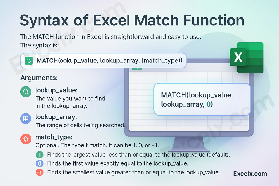
The syntax is:
=MATCH(lookup_value, lookup_array, [match_type])
Arguments:
- lookup_value: The value you want to find in the lookup_array.
- lookup_array: The range of cells being searched.
- match_type: Optional. The type of match. It can be 1, 0, or -1.
- 1: Finds the largest value less than or equal to the lookup_value (default).
- 0: Finds the first value exactly equal to the lookup_value.
- -1: Finds the smallest value greater than or equal to the lookup_value.
Practical Uses of the MATCH Function
MATCH function in Excel is used to locate the position of a specific value within a given range or array. It enables precise dynamic lookups, making it ideal for error handling, advanced calculations, and comprehensive data analysis. It is designed to search for a value and return its relative position in complex lookup formulas. It’s particularly useful for:
- Dynamic Data Retrieval: Finding the position of a value dynamically within a dataset.
- Complex Lookups: Enhancing lookup operations when combined with other functions like INDEX.
- Data Validation: Ensuring that values exist within a specified range.
- Conditional Calculations: Performing calculations based on the position of values in arrays.
By leveraging these capabilities, you can enhance your data analysis, reporting, and calculation efforts, making the MATCH function a vital tool in your Excel toolkit.
How to Use the MATCH Function?
The MATCH function in Excel is versatile and can be used in various ways depending on the requirement. Below, we’ll walk you through the basic steps and some practical examples to help you get started with the MATCH function.
Step-by-Step Guide to Using the MATCH Function
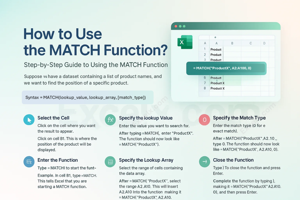
Let’s walk through the steps of using the MATCH function with a practical example. Suppose we have a dataset containing a list of product names, and we want to find the position of a specific product.
- Select the Cell
- Action: Click on the cell where you want the result to appear.
- Example: Click on cell B1. This is where the position of the product will be displayed.
- Enter the Function
- Action: Type =MATCH( to start the function.
- Example: In cell B1, type =MATCH(. This tells Excel that you are starting a MATCH function.
- Specify the Lookup Value
- Action: Enter the value you want to search for.
- Example: After typing =MATCH(, enter “ProductX”. The function should now look like =MATCH(“ProductX”.
- Specify the Lookup Array
- Action: Select the range of cells containing the data array.
- Example: After =MATCH(“ProductX”,, select the range A2: A10. This will insert A2:A10 into the function, making it =MATCH(“ProductX”, A2:A10.
- Specify the Match Type
- Action: Enter the match type (0 for exact match).
- Example: After =MATCH(“ProductX”, A2:A10,, type 0. The function should now look like =MATCH(“ProductX”, A2:A10, 0).
- Close the Function
- Action: Type ) to close the function and press Enter.
- Example: Complete the function by typing ), making it =MATCH(“ProductX”, A2:A10, 0), and then press Enter.
Outcome: The cell B1 will now display the position of “ProductX” within the range A2:A10.
Example in Context
- Select the Cell: Click on cell B1
- Enter the Function: Type =MATCH(
- Specify the Lookup Value: Enter “ProductX”
- Specify the Lookup Array: Select the range A2:A10
- Specify the Match Type: Enter 0
- Close the Function: Type ) and press Enter
By following these steps, you can easily use the MATCH function to find the relative position of values within a range in Excel.
Practical Examples of the Excel MATCH Function
The MATCH function in Excel is incredibly versatile and can be applied in various scenarios to streamline your data retrieval tasks. Below is a table of practical examples that illustrate how to use the MATCH function for different purposes, ranging from simple lookups to more complex data analysis. These examples will help you understand how to leverage the MATCH function to enhance your productivity and efficiency in Excel.

| Example | Description | Formula | Result |
|---|---|---|---|
| Finding the Position of a Product | Searches for a product name and returns its position. | =MATCH(“ProductX”, A2:A100, 0) | Position of “ProductX” in the range A2:A100. |
| Finding the Position of a Number | Searches for a number and returns its position in a numeric array. | =MATCH(100, B2:B100, 0) | Position of the number 100 in the range B2:B100. |
| Approximate Match | Finds the largest value less than or equal to the lookup value (array must be sorted ascending). | =MATCH(50, C2:C100, 1) | Position of the closest match to 50 in C2:C100. |
| Finding the Position of a Date | Searches for a specific date and returns its position. | =MATCH(“2024-01-01”, D2:D100, 0) | Position of the date “2024-01-01” in D2:D100. |
| Two-Way Lookup with MATCH and INDEX | Combines MATCH with INDEX for a two-way lookup. | =INDEX(A2:Z100, MATCH(“ProductX”, A2:A100, 0), MATCH(“Sales”, A1:Z1, 0)) | Value at the intersection of “ProductX” (row) and “Sales” (column). |
| Finding the Smallest Value | Finds the smallest value greater than or equal to the lookup value (range must be sorted descending). | =MATCH(25, E2:E100, -1) | Position of the smallest value ≥ 25 in E2:E100. |
| Dynamic Column Reference | Uses MATCH to dynamically reference a column for VLOOKUP. | =VLOOKUP(“ProductX”, A2:D100, MATCH(“Sales”, A1:D1, 0), FALSE) | Sales value for “ProductX”. |
| Finding the Position in a Horizontal Array | Searches for a value in a horizontal range and returns its position. | =MATCH(“Jan”, F1:K1, 0) | Position of “Jan” in the range F1:K1. |
| Conditional Lookup | Uses MATCH with IF to perform a conditional lookup. | =IF(G1=”Yes”, MATCH(“ProductY”, A2:A100, 0), “Not Applicable”) | Position of “ProductY” if G1 equals “Yes”. |
| Finding Text in a Mixed Array | Searches for text within a mixed data type array and returns its position. | =MATCH(“CategoryA”, H2:H100, 0) | Position of “CategoryA” in the range H2:H100. |
Download Example File
Ready to put your Excel MATCH skills to the test? Download our free example file that includes a comprehensive dataset along with practical formulas and step-by-step instructions. This practice workbook will help you reinforce your understanding of the MATCH function and related lookup techniques. Click the link below to get started and boost your Excel proficiency!
Excel MATCH Function: Best Practices for Effective Use
To maximize the effectiveness of the MATCH function in Excel, it’s essential to follow best practices that ensure accuracy, efficiency, and ease of maintenance. This section provides practical tips and strategies to help you leverage the MATCH function to its fullest potential, whether you’re working with simple lookups or more complex data retrieval tasks. By adhering to these guidelines, you can enhance your productivity and maintain the integrity of your data.
- Combine with INDEX: Enhance the utility of MATCH by combining it with the INDEX function to create dynamic and flexible lookups. This combination allows you to locate the row and column numbers dynamically.
- Use Exact Match for Precision: For most lookup tasks, use an exact match (match_type = 0) to ensure accurate results. Approximate matches (match_type = 1 or -1) can lead to unexpected results if the data is not sorted.
- Handle Errors Gracefully: Incorporate error handling functions such as IFERROR to manage potential errors gracefully. For example,
IFERROR(MATCH("ProductX", A2:A110, 0), "Not Found")can help handle cases where the lookup value is not found.
- Document Your Formulas: Add comments or documentation within your Excel workbook to explain complex formulas. This helps others understand your logic and makes it easier for you to revisit your work later.
- Test with Sample Data: Before applying the MATCH function to a large dataset, test it with a small sample to ensure it behaves as expected. This can help identify potential issues early.
- Combine with Other Functions: Use MATCH with other functions like VLOOKUP, HLOOKUP, and OFFSET to perform more complex data retrieval tasks.
- Regular Updates and Reviews: Periodically review and update your formulas and data to ensure they remain accurate and relevant. This is especially important if your data changes frequently.
- Optimize for Performance: Avoid using excessively large ranges to maintain optimal performance. Break down complex lookups into smaller, manageable parts if necessary.
- Stay Updated on Excel Features: Microsoft regularly updates Excel with new features and functions. Stay informed about these updates as they can provide new tools and techniques to enhance your use of the MATCH function.
Related Functions
The MATCH function is part of a family of lookup and reference functions in Excel that are designed to perform complex data retrieval and analysis. Understanding these related functions can help you perform more advanced data tasks by combining them with MATCH or using them as alternatives. Here’s a look at some key related functions:
| Function | Description | Usage with MATCH | Example |
|---|---|---|---|
| INDEX Function | Returns the value of an element in a table or array, selected by the row and column number indexes. | Use MATCH to dynamically find row and column numbers for INDEX. |
=INDEX(A2:Z100, MATCH(E1, A2:A100, 0), MATCH(F1, A1:Z1, 0)) |
| VLOOKUP Function | Searches for a value in the first column of a range and returns a value in the same row from a specified column. | Use MATCH to dynamically determine the column number for VLOOKUP. |
=VLOOKUP(G1, A2:D100, MATCH("Sales", A1:D1, 0), FALSE)
|
| HLOOKUP Function | Searches for a value in the first row of a range and returns a value in the same column from a specified row. | Use MATCH to dynamically determine the row number for HLOOKUP. |
=HLOOKUP(H1, A1:Z100, MATCH("Category", A1:A100, 0), FALSE)
|
| OFFSET Function | Returns a reference to a range that is a specified number of rows and columns from a cell or range of cells. | Use MATCH to define dynamic offsets for data retrieval. |
=OFFSET(A1, MATCH("ProductX", A2:A100, 0), MATCH("Sales", A1:Z1, 0))
|
| CHOOSE Function | Returns a value from a list of values based on an index number. | Use MATCH to dynamically select values from a list. |
=CHOOSE(MATCH("Q1", {"Q1","Q2","Q3","Q4"}, 0), 100, 200, 300, 400)
|
| LOOKUP Function | Searches for a value in a vector or array and returns a value in the same position from another vector or array. | Use LOOKUP for simpler lookup tasks that don’t require MATCH’s flexibility. |
=LOOKUP(J1, A2:A100, B2:B100) |
| MATCH Function | Returns the relative position of an item in an array that matches a specified value in a specified order. | Use MATCH to find positions dynamically for other functions. |
=MATCH(K1, L2:L100, 0) |
Frequently Asked Questions about the Excel MATCH Function
Understanding the MATCH function and its related queries can greatly enhance your ability to manipulate and analyze data in Excel. By mastering the following FAQs, you’ll be better equipped to handle various data retrieval tasks efficiently.
- What is the MATCH function in Excel?
-
- The MATCH function in Excel searches a specified range for a particular value and returns its relative position within that range.
- How do I use the MATCH function?
-
- The syntax for the MATCH function is:
MATCH(lookup_value, lookup_array, [match_type])
. Example:
=MATCH("ProductX", A2:A10, 0)searches for “ProductX” and returns its position in A2:A10.
- The syntax for the MATCH function is:
- What are the different match types in the MATCH function?
-
- The MATCH function has three match types: 1 (largest value less than or equal to lookup_value), 0 (exact match), and -1 (smallest value greater than or equal to lookup_value).
- Can the MATCH function handle non-numeric data?
-
- Yes, the MATCH function can handle text, numbers, and dates. It searches for the specified value within the lookup_array and returns its position.
- How can I combine the MATCH function with INDEX for dynamic lookups?
-
- Combine MATCH with INDEX to dynamically find the row and column numbers. Example:
=INDEX(A2:A10, MATCH(E1, A2:A10, 0), MATCH(F1, A1:A10, 0))
retrieves the value where the row matches E1 and the column matches F1.
- Combine MATCH with INDEX to dynamically find the row and column numbers. Example:
- What common errors should I watch out for when using the MATCH function?
-
- The most common error is #N/A, which occurs if the lookup_value is not found in the lookup_array. Ensure the value exists and use the correct match type.
- How can I use the MATCH function with named ranges?
-
- Use named ranges to simplify your formulas. Example:
=MATCH("ProductX", ProductList, 0)searches for “ProductX” in the named range “ProductList”.
- Use named ranges to simplify your formulas. Example:
- Can the MATCH function be used for two-way lookups?
-
- Yes, combine MATCH with INDEX for two-way lookups. Example:
=INDEX(A2AA10, MATCH(H1, A2:A10, 0), MATCH(I1, A1:A10, 0))
retrieves the value where the row matches H1 and the column matches I1.
- Yes, combine MATCH with INDEX for two-way lookups. Example:
- How do I use the MATCH function for approximate matches?
-
- Use match_type 1 or -1 for approximate matches. Example:
=MATCH(50, A2:A10, 1)
finds the largest value less than or equal to 50 in A2:A10.
- Use match_type 1 or -1 for approximate matches. Example:
- What are some advanced uses of the MATCH function?
-
- Advanced uses include dynamic column references for VLOOKUP, conditional lookups with IF, and integration with OFFSET for complex data retrieval.
Conclusion
Mastering the Excel MATCH function unlocks powerful capabilities for dynamic data retrieval, advanced lookups, and complex calculations. We’ve explored how to find the relative position of values, understand its syntax, explore diverse uses, practical examples, best practices, and common FAQs. By implementing these insights, you can significantly enhance your efficiency and productivity in Excel. Embrace the MATCH function to optimize your Excel skills and achieve better results.
