Table of Contents

Excel keyboard shortcuts for filtering data are essential tools for anyone looking to streamline their workflow and work more efficiently. When dealing with large datasets, filtering allows you to quickly narrow down the data you need, whether it’s project tasks, sales figures, or customer information. By applying filters, you can focus only on the most relevant rows, saving valuable time and ensuring you’re working with the data that matters.
Mastering these shortcuts will significantly boost your productivity. Instead of manually navigating through menus, you can use simple keystrokes to apply, modify, and clear filters, making the entire process quicker and more efficient. In this blog post, we’ll guide you through the most essential Excel filtering shortcuts, with practical examples to help you improve your data analysis and management.
What is Data Filtering in Excel?
Data filtering in Excel is a technique used to display only specific rows of data based on the criteria you set, while hiding others. This allows you to quickly find and analyze the data you need. You can filter data by numbers, text, dates, or even by cell color, enabling you to create targeted views of your data without modifying or deleting any information.
Key Concepts:
- Column headers: These represent the field names you want to filter.
- Filter criteria: Filters are applied based on the condition you specify (e.g., greater than a certain number, or specific text).
- Dropdown menu: Filter options are presented as dropdown menus in the header cells.
Why Do We Need to Filter Data?
Filtering data is an essential task for anyone who works with large datasets. It allows users to display only the rows that meet certain criteria, making it easier to focus on relevant data and perform detailed analysis. Whether you’re managing a project, tracking sales, or analyzing customer data, filtering helps you:
- Isolate Relevant Information: Quickly focus on the data that matters.
- Enhance Data Analysis: Organize your dataset to analyze trends, identify patterns, and make informed decisions.
- Improve Efficiency: Avoid unnecessary scrolling through irrelevant data, saving you time.
Without filters, you would be forced to sift through thousands of rows manually. But with filters, you can immediately see what’s important, making data management much more manageable.
Excel Shortcut Key for Filtering Data
Mastering Excel’s filtering shortcut keys is crucial for those looking to optimize their workflows and reduce the amount of time spent on repetitive tasks. The right shortcut can help you apply, remove, and navigate filters with ease. Below is a table summarizing the essential filtering shortcuts in Excel to filter data efficiently:
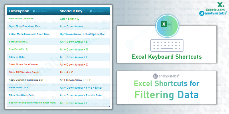
| Description | Shortcut Key |
|---|---|
| Turn Filters On or Off | Ctrl + Shift + L |
| Open Filter Dropdown Menu | Alt + Down Arrow |
| Select Menu Items with Arrow Keys | Up/Down Arrow, Enter/Space Bar |
| Sort Data (A to Z) | Alt + Down Arrow + S |
| Sort Data (Z to A) | Alt + Down Arrow + O |
| Filter by Color | Alt + Down Arrow + I |
| Clear Filters for a Column | Alt + Down Arrow + C |
| Clear All Filters in a Range | Alt + A + C |
| Apply Custom Filter Dialog Box | Alt + Down Arrow + F + E |
| Filter Blank Cells | Alt + Down Arrow + F + E + Enter |
| Filter Non-Blank Cells | Alt + Down Arrow + F + N + Enter |
| Search for a Specific Value in Filter Menu | Alt + Down Arrow + E |
These shortcuts help you navigate through filters quickly and efficiently, allowing you to manage large datasets with ease.
How to Filter in Excel using Shortcuts?
Using Excel keyboard shortcuts to filter data can significantly speed up your workflow and make data analysis more efficient. There are several useful Excel filter shortcuts available that allow you to turn on filters, access filter menus, clear filters, and perform advanced filtering operations. Here’s a comprehensive list of shortcuts to help you filter data with ease:
Basic Filtering Shortcuts
- Turn Filters On or Off: Ctrl + Shift + L, Toggles the filter feature on or off for the selected range, adding or removing filter dropdowns in the header.
- Open Filter Dropdown Menu: Alt + Down Arrow, Opens the dropdown menu for the selected column, allowing you to apply or modify the filter.
- Apply Filter Using Arrow Keys: Up/Down Arrow, Enter, Spacebar, Use the arrow keys to navigate through filter options, press Enter to apply, or Spacebar to check/uncheck items.
- Sort Data A to Z: Alt + Down Arrow + S, Sorts the selected column data in ascending (A to Z) order.
- Sort Data Z to A: Alt + Down Arrow + O, Sorts the selected column data in descending (Z to A) order.
- Clear Filters for a Column: Alt + Down Arrow + C, Clears the filter applied to a specific column, resetting it to show all data.
- Clear All Filters in Range: Alt + A + C, Clears all filters applied to the current range, restoring the full dataset.
- Filter by Color: Alt + Down Arrow + I, Filters data based on cell or font color, useful for color-coded data.
- Filter for Blank Cells: Alt + Down Arrow + F + E + Enter, Filters for blank cells in the selected column.
- Filter for Non-Blank Cells: Alt + Down Arrow + F + N + Enter, Filters for non-blank cells in the selected column.
- Show Only Visible Cells: Alt + ; (semicolon), Selects only the visible cells in a filtered range, excluding hidden rows.
- Apply Filter for Multiple Columns: Ctrl + Shift + L, Turn on filter for multiple columns by selecting all columns and pressing the shortcut.
Advanced Filtering Shortcuts
- Filter by Text Criteria: Alt + Down Arrow + F + E, Opens the custom filter dialog box for filtering text-based data using criteria like “contains”, “equals”, etc.
- Filter by Date Range: Alt + Down Arrow + F + D, Filters data based on a date range (e.g., before, after, or between dates).
- Filter for Top 10 Values: Alt + Down Arrow + F + T, Filters and displays the top N values in the column, based on your specified number (e.g., Top 3, Top 10).
- Apply Custom Filter (Greater Than, Less Than, etc.): Alt + Down Arrow + F + E, Opens the custom filter dialog to apply advanced filters such as “greater than”, “less than”, “contains”, and other custom conditions.
- Search for Specific Value in Filter Menu: Alt + Down Arrow + E, Opens the search box within the filter menu, allowing you to quickly search for a specific value.
- Filter Using Wildcards: Alt + Down Arrow + F + E, Apply filters with wildcard characters (e.g., * for any sequence of characters, ? for a single character).
- Filter for Bottom 10 Values: Alt + Down Arrow + F + B, Filters and displays the bottom N values based on your specified number (e.g., Bottom 5, Bottom 10).
- Filter by Multiple Criteria: Alt + Down Arrow + F + E, Use this to filter data with multiple conditions (e.g., filter by greater than and less than simultaneously).
- Filter Using Custom Date Filters: Alt + Down Arrow + F + D, Use custom filters such as “This Week”, “Next Month”, or specific date ranges.
- Filter for Items Containing Specific Text: Alt + Down Arrow + F + C, Filters data by selecting items that contain specific text.
Data Range and Column-Specific Shortcuts
- Filter for Unique Values: Alt + Down Arrow + F + U, Filters and displays only unique values in a selected column.
- Reapply Filters: Ctrl + Alt + L, Reapplies the last filter used, useful after making changes to the data.
- Expand Filter Selection: Ctrl + Shift + Arrow Key, Expands the selected range to include the entire data set for applying filters.
- Clear Filter from All Columns: Ctrl + Shift + L, Press again to remove all filters from all columns at once.
- Select Column for Filtering: Ctrl + Spacebar, Selects the entire column to apply the filter.
- Move to the Next Filtered Row: Alt + Down Arrow + F + N, Move to the next row that matches the filter criteria.
Navigation and Interaction Shortcuts
- Jump to Filter Search Box: Alt + Down Arrow + E, Takes you directly to the search box within the filter dropdown for quick filtering.
- Select All in Filter: Spacebar, In the filter dropdown, pressing the spacebar selects or deselects the “Select All” checkbox.
- Move Through Filter Options: Up/Down Arrow, Use to navigate through items in the filter dropdown.
- Apply Filter from Search Box: Enter, After typing in the search box, press Enter to apply the filter based on your search criteria.
- Toggle Filter Selection in Menu: Spacebar, Check or uncheck items in the filter dropdown using the spacebar.
- Jump to First Filter Item: Home, Navigate to the first item in the filter dropdown list.
- Jump to Last Filter Item: End, Navigate to the last item in the filter dropdown list.
- Page Up/Down in Filter List: Page Up, Page Down, Scroll through large filter lists by one screen at a time.
Filtering Data by Specific Conditions
- Filter for Numeric Values Greater Than: Alt + Down Arrow + F + E, Apply a custom filter for values greater than a specified number.
- Filter for Numeric Values Less Than: Alt + Down Arrow + F + E, Apply a custom filter for values less than a specified number.
- Filter for Specific Date: Alt + Down Arrow + F + D, Filter for data corresponding to a specific date.
- Filter by Custom Date Criteria: Alt + Down Arrow + F + D, Filter by custom date conditions like “last month” or “next week”.
- Filter for a Specific Number Range: Alt + Down Arrow + F + N, Filters the data to show numbers within a specified range.
- Filter for Specific Text Using “Contains”: Alt + Down Arrow + F + C, Filter by text criteria such as “contains” certain words.
- Filter for Data That Begins With Specific Text: Alt + Down Arrow + F + B, Filters for data that starts with specific text.
- Filter for Data That Ends With Specific Text: Alt + Down Arrow + F + E, Filters for data that ends with specific text.
- Filter for Blank or Non-Blank Cells: Alt + Down Arrow + F + E, Choose to filter blank or non-blank cells in the selected column.
Special Filtering Shortcuts
- Filter for Multiple Values: Alt + Down Arrow + F + M, Apply a filter for multiple values in a column.
- Filter for a Date Range: Alt + Down Arrow + F + R, Filter data based on a custom date range.
- Apply Text Filter for Case Sensitivity: Alt + Down Arrow + F + A, Apply a text filter that differentiates between uppercase and lowercase letters.
- Filter for Data Using a Formula: Alt + Down Arrow + F + F, Use this to filter data based on formula results (e.g., filtering rows where a certain formula returns true).
- Toggle Visibility of Filtered Data: Ctrl + Shift + 9, Unhides hidden rows in a filtered dataset.
How to Turn Filters On or Off in Excel
Enabling filters in Excel is easy, and it’s an essential first step before you can start filtering data. By turning on filters, Excel adds dropdown arrows to each column header, allowing you to apply different filters to each column.
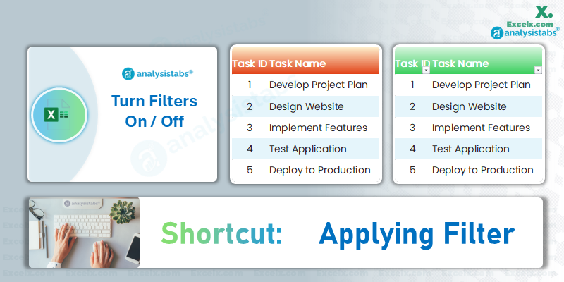
Shortcut: Ctrl + Shift + L
Steps:
- Select any cell within your data range.
- Press Ctrl + Shift + L to enable filters. If filters are already applied, the same shortcut will remove them.
The shortcut Ctrl + Shift + L toggles the filter feature on and off for your selected data range. When filters are turned on, dropdown arrows appear in the header cells, allowing you to filter data as needed.
Example Scenario: Filtering Tasks by Status
Imagine you have a project management task table, and you want to filter tasks by their status (e.g., In Progress or Completed).
- Step 1: Select a cell within your data range.
- Step 2: Press Ctrl + Shift + L to turn on the filter feature. Dropdown arrows will appear in the header row.
- Step 3: Use the dropdown in the Status column to filter tasks by status.
This shortcut streamlines the process of applying filters, ensuring you can quickly focus on the relevant data.
How to Open the Filter Dropdown Menu
Once filters are turned on, you’ll want to access the filter options in each column. To open the dropdown menu for a specific column, use the shortcut Alt + Down Arrow.
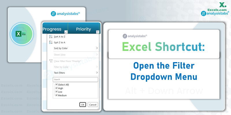
Shortcut to Open the Filter Dropdown Menu:
- Alt + Down Arrow
Once filters are applied, use Alt + Down Arrow to open the dropdown menu of the selected column. This shortcut lets you access various filtering options without using your mouse.
Example Scenario: Filtering Tasks by Priority
For instance, you may want to view only the “High Priority” tasks from the Priority column.
- Step 1: Select the Priority column header.
- Step 2: Press Alt + Down Arrow to open the filter menu.
- Step 3: Choose “High” from the dropdown to filter the tasks.
This shortcut is incredibly useful for quickly accessing the filter menu for any column.
How to Sort Data in Excel Using Filters (A to Z or Z to A)
Sorting your data can help organize it in a logical sequence. Excel allows you to sort data either in ascending or descending order using the filter dropdown.
Shortcuts to Sort Data in Excel Using Filters:
- Alt + Down Arrow + S (Sort A to Z)
- Alt + Down Arrow + O (Sort Z to A)
These shortcuts allow you to sort data alphabetically or numerically within the selected column. Use S to sort from A to Z, and O to sort from Z to A.
Example Scenario: Sorting Tasks by Progress
You want to sort your tasks by progress, from the least completed to the most completed.
- Step 1: Select the Progress column header.
- Step 2: Press Alt + Down Arrow + S to sort the tasks from least to most completed.
How to Filter by Color
You can filter data based on cell color or font color, which is useful when you use conditional formatting to categorize data visually.
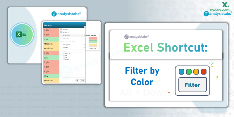
Shortcut Filter by Color:
- Alt + Down Arrow + I
This shortcut allows you to filter data based on cell or font color, which is helpful when you’re working with conditional formatting or visual categorization.
Example Scenario: Filtering High Priority Tasks by Color
Let’s say you color-coded your tasks with a red fill for “High” priority.
- Step 1: Select the Priority column header.
- Step 2: Press Alt + Down Arrow + I to open the filter by color submenu.
- Step 3: Choose the color (e.g., red) to filter all high-priority tasks.
This shortcut saves time when filtering tasks that are visually marked.
How to Apply Custom Filter in Excel
The Custom Filter Dialog allows you to filter data based on more complex conditions, such as “greater than”, “less than”, “contains”, or “does not equal”. This feature is great when you need to apply multiple filtering criteria to a column.
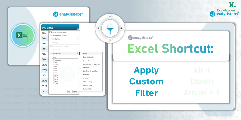
Shortcut to Apply Custom Filter:
- Alt + Down Arrow + F + E
Example:
To filter for tasks that have a Progress greater than 50%:
- Open the dropdown for the Progress column.
- Press Alt + Down Arrow + F + E to open the custom filter dialog.
- Set the condition “greater than” and enter 50%.
How to Filter for Blank or Non-Blank Cells
You can filter for blank or non-blank cells in a column to identify missing or incomplete data.
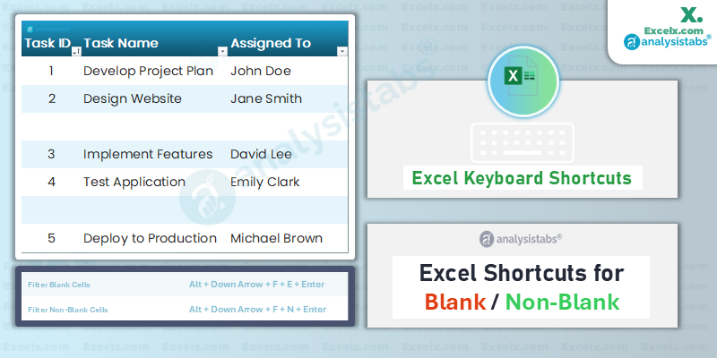
Shortcuts Filter for Blank or Non-Blank Cells:
- Alt + Down Arrow + F + E + Enter (Filter Blank Cells)
- Alt + Down Arrow + F + N + Enter (Filter Non-Blank Cells)
Use these shortcuts to filter out blank or non-blank cells in a column.
Example Scenario: Filtering Blank End Dates
If you need to see tasks that still lack an end date, use the following:
- Step 1: Select the End Date column.
- Step 2: Press Alt + Down Arrow + F + E + Enter to filter blank cells.
- Step 3: The table will show only tasks that do not have an end date.
How to Clear Filters for a Column
If you want to remove the filter from a single column, you can use the C key after opening the filter menu.
Shortcut to Clear Filters for a Column:
- Alt + Down Arrow + C
Example:
To clear the filter in the Priority column:
- Open the dropdown menu by pressing Alt + Down Arrow.
- Press C to clear the filter.
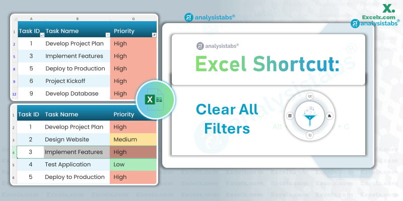
How to Clear All Filters
To remove all applied filters at once, you can use the Alt + A + C shortcut. This will reset the data, showing all rows in the worksheet.
Shortcut to Clear All Filters:
- Alt + A + C
Shortcut Key for Removing Filter in Excel
Removing filters in Excel can be done easily using the following shortcut keys:
- Alt + Down Arrow + C – Clear Filter for a Column
Clears the filter applied to a specific column, restoring the view to show all data in that column. - Alt + A + C – Clear All Filters
Clears all filters applied to the data range or worksheet, showing all rows and columns.
These shortcuts help you quickly reset your data and remove filters without needing to navigate through menus, making your workflow more efficient.
How to Filter Top Values
To display only the top values in a column, you can filter using the “Top 10” feature. This is particularly useful when analyzing top-performing products, highest sales figures, or top priority tasks.
Shortcut: Alt + Down Arrow + F + T
Example:
To display the top 3 tasks with the highest Progress:
- Open the filter dropdown in the Progress column.
- Press Alt + Down Arrow + F + T to open the top values filter.
- Enter 3 in the dialog box to filter for the top 3 values.
How to Use Search Box in Filter Menu
If you have a long list of items in your filter dropdown, you can quickly locate a specific value using the search box.
Shortcut: Alt + Down Arrow + E
Example:
- Step 1: Open the filter menu by pressing Alt + Down Arrow.
- Step 2: Press E to jump to the search box.
- Step 3: Type the value you’re looking for (e.g., “In Progress”).
Shortcut key for Sort and Filter in Excel
Excel provides several handy shortcuts that make sorting and filtering data much more efficient. These shortcuts save you from navigating through the ribbon menus and allow you to quickly apply sorting or filtering options to your data. Here are the most essential shortcuts for sorting and filtering in Excel:
- Alt + Down Arrow + S – Sort A to Z (Sorts data in ascending order)
- Alt + Down Arrow + O – Sort Z to A (Sorts data in descending order)
- Alt + Down Arrow + T – Sort by Color sub-menu (Sorts data based on color)
- Alt + Down Arrow + I – Filter by Color sub-menu (Filters data by color)
- Alt + Down Arrow + F – Text or Date Filter sub-menu (Applies text or date-based filters)
- Alt + Down Arrow + E – Open Search Box in Filter (Allows you to search within the filter menu)
- Alt + Down Arrow + A – Apply all filter criteria (Applies all set filter options)
- Alt + Down Arrow + C – Clear filter (Clears the filter for the selected column)
Shortcut Key for Drop-Down List in Excel
Excel makes it easy to use drop-down lists for data validation, and there are shortcuts that can help you interact with these lists more efficiently. Here’s a list of the key shortcuts to access and use drop-down lists in Excel:
- Alt + Down Arrow – Open Drop-Down List
Opens the drop-down list for a cell with data validation, allowing you to select an option from the list. - Up/Down Arrow – Navigate Through Drop-Down List
Use the Up and Down Arrow keys to scroll through the available options in a drop-down list. - Enter – Select an Option
After highlighting the desired option in the drop-down list, press Enter to select it. - Esc – Close Drop-Down List
Press Esc to close the drop-down list without making any selection. - Alt + Down Arrow + E – Open Search Box in Drop-Down List
In a drop-down list with a search feature, this shortcut allows you to jump to the search box where you can type your search term.
These shortcuts are especially helpful for quickly navigating and selecting options from drop-down lists, improving the efficiency of data entry in Excel.
How to Filter Multiple Criteria
Excel allows you to filter data based on multiple conditions across different columns. Here’s how you can filter using multiple conditions:
- Apply Filters: Select your data and press Ctrl + Shift + L to enable the filter.
- Set Conditions for Multiple Columns:
- For Column 1: Filter based on “Contains” or “Greater than”.
- For Column 2: Filter based on specific dates or numbers.
- For Column 3: Apply another condition, such as text matching.
Excel will display rows that meet all the filter conditions across the columns.
Example:
You can combine multiple filters across different columns to narrow down your dataset even further. For instance, you might want to filter tasks that are both “In Progress” and have a “High” priority.
- Step 1: Apply a filter for Status as “In Progress”.
- Step 2: Apply another filter for Priority as “High”.
These combined filters will help you focus on the most critical tasks.
How to Copy Filtered Data
After applying a filter, you may want to copy and paste the visible data while excluding the hidden rows. This can be done easily with a few steps.
Steps:
- Select the visible data.
- Press Ctrl + C to copy.
- Go to the location where you want to paste and use Ctrl + V.
How to Filter 3 Columns in Excel?
Filtering multiple columns in Excel simultaneously is very straightforward. Here’s how you can filter three columns at once:
- Apply Filter: Select your data range and press Ctrl + Shift + L to apply filters to all columns.
- Choose Criteria for Each Column:
- For Column 1: Use the dropdown to filter by the desired criteria.
- For Column 2: Apply a filter, such as “Greater Than”, to select specific values.
- For Column 3: Choose “Contains” to search for certain text.
Excel will then filter the data based on your selections for all three columns simultaneously.
What is the Top 10 Filter in Excel?
The “Top 10” filter in Excel allows you to quickly filter and display the top N items in a dataset based on numerical values, making it ideal for ranking or identifying the highest/lowest performing records. Here’s how to use it:
- Open Filter Menu: Click the dropdown in the column you want to filter.
- Select Top 10 Filter: Choose “Top 10” from the menu.
- Set Criteria: Enter the number of items to show (e.g., Top 5, Top 10).
This filter is widely used for sales, performance metrics, and other ranked data.
How to Use Filter Formula in Excel?
Excel offers powerful formula-based filters like the FILTER() function, allowing users to filter data dynamically within formulas. This can be used to extract data based on specific conditions without manually applying filters. Here’s how to use the formula:
- Syntax: =FILTER(array, include, [if_empty])
- Example: To filter all tasks where the progress is greater than 50%:
=FILTER(A2:B10, B2:B10>50)
- Dynamic Results: The result will update automatically as data changes.
This formula-based approach makes your filtering more flexible and dynamic.
How Do I Add a Filter to a Dropdown?
To add a filter to a dropdown in Excel, you’ll need to set up a drop-down list first, and then apply a filter to that list. Here’s how to do it:
- Create a Dropdown: Use Data Validation to create a drop-down list.
- Select the cell.
- Go to the Data tab > Data Validation > List.
- Apply Filter: Once the drop-down is created, turn on the filter using Ctrl + Shift + L, and the dropdown filter will appear.
- Filter Data: Use the dropdown to filter based on the selected value.
This combination allows you to filter data by selecting an option from the drop-down.
How to Filter in Excel by Name?
Filtering data by name in Excel is useful when you need to find or highlight rows containing specific names. Here’s how you can filter by name:
- Enable Filters: Press Ctrl + Shift + L to turn on filters.
- Select the Name Column: Click on the filter dropdown in the column that contains the names.
- Search for a Name: Type the name into the search box within the filter dropdown and select it.
This method is helpful for quickly locating specific entries like employees, customers, or products by name.
How to Filter Data Using Text Criteria in Excel?
You can filter data based on specific text criteria such as “Contains”, “Begins with”, or “Equals”. Here’s how:
- Select Column: Click on the dropdown in the column you want to filter.
- Choose Text Filters: Choose the Text Filters option from the dropdown menu.
- Select Criteria: Choose your condition (e.g., Contains, Equals).
- Enter Text: Type the specific text you want to filter for and click OK.
This filter is ideal when dealing with names, addresses, or any other text-based data.
How to Filter Data by Date Range in Excel?
Filtering by date range is an essential feature when working with time-based data like project timelines, sales records, or financial data. Here’s how you can filter by date:
- Click the Date Column: Select the column containing dates.
- Open Date Filters: Click the dropdown and select Date Filters.
- Set a Date Range: Choose from options like “Between”, “Before”, or “After” to filter by specific date ranges.
This functionality helps in narrowing down data to specific periods like months, years, or days.
How to Filter Unique Values in Excel?
Excel has a feature that lets you filter unique values to identify distinct records. Here’s how:
- Select Data Range: Highlight the range you want to filter.
- Apply Filter: Enable the filter using Ctrl + Shift + L.
- Select Unique Values: In the filter dropdown, click on the filter options and choose Unique or Distinct (depending on your Excel version).
This is perfect for identifying unique entries in a dataset, such as unique products, customer IDs, or cities.
How to Use Advanced Filter in Excel?
Advanced Filter in Excel allows you to filter data based on complex conditions, including multiple criteria or even wildcard characters. Here’s how to use it:
- Set Criteria Range: Define the criteria in a separate range of cells.
- Go to Data Tab: Click on Advanced in the Sort & Filter group.
- Choose Criteria: Select the data range and set the criteria range.
- Apply Filter: Click OK to filter the data based on the specified criteria.
This method is useful for applying complex filters that are not available with regular filter options.
Advanced Filter Shortcut Key in Excel
While Excel doesn’t have a direct single shortcut for accessing the Advanced Filter dialog, you can use a combination of keyboard shortcuts to open and apply advanced filters. Here’s how to access it efficiently:
- Alt + D + F + A – Open Advanced Filter Dialog
This opens the “Advanced Filter” dialog box, allowing you to apply complex filtering criteria such as multiple conditions or filtering based on a different criteria range.- You can use this to filter data with more complex conditions, such as using criteria from another range or applying logical operators like AND/OR.
Example:
- Steps to use the Advanced Filter:
- Press Alt + D + F + A to open the Advanced Filter dialog box.
- Select your data range and criteria range.
- Choose whether to filter the data in place or copy it to another location, then click OK.
The Advanced Filter provides more flexibility than regular filters, allowing for complex queries and conditions.
Filtering Data Using VBA
When working with large datasets in Excel, applying filters manually can be time-consuming. Thankfully, VBA (Visual Basic for Applications) offers a powerful way to automate this process, making it faster and more efficient. By using VBA code to filter your data, you can quickly sort through specific rows, focus on relevant information, and remove unnecessary clutter. In this section, we’ll explore some useful VBA codes to filter data based on various criteria, such as values, dates, and custom conditions, allowing you to streamline your data analysis tasks.
Apply Filter to a Range
This VBA code applies a filter to a specific range based on a given criteria.
Sub ApplyFilter()

Dim ws As Worksheet
Set ws = ThisWorkbook.Sheets("Sheet1")

' Apply filter on the first column (A) for "Completed" status

ws.Range("A1").AutoFilter Field:=1, Criteria1:="Completed"
End Sub
- What it does: Applies a filter to the first column (A) where the values match “Completed”.
Apply Multiple Filters
This code applies multiple filters to a range of data for different columns.
Sub ApplyMultipleFilters()

Dim ws As Worksheet
Set ws = ThisWorkbook.Sheets("Sheet1")


' Apply filter on column A for "In Progress" and column B for "High Priority"
ws.Range("A1:B1").AutoFilter Field:=1, Criteria1:="In Progress"
ws.Range("A1:B1").AutoFilter Field:=2, Criteria1:="High Priority"

End Sub
- What it does: Applies a filter to multiple columns, showing only rows with “In Progress” in column A and “High Priority” in column B.
Clear Filter from a Specific Column
This VBA code removes the filter from a specific column.
Sub ClearFilter()

Dim ws As Worksheet
Set ws = ThisWorkbook.Sheets("Sheet1")


' Clear filter from column A
ws.AutoFilterMode = False

End Sub
- What it does: Clears any applied filter in the entire worksheet.
Apply Custom Filter (Greater Than)
This VBA code applies a custom filter with a condition like “greater than” a specified value.
Sub CustomFilterGreaterThan()

Dim ws As Worksheet
Set ws = ThisWorkbook.Sheets("Sheet1")


' Apply filter where values in column B are greater than 50
ws.Range("A1:B1").AutoFilter Field:=2, Criteria1:=">50"

End Sub
- What it does: Filters column B to show only values greater than 50.
Filter Data by Date Range
This code applies a date range filter to a column.
Sub DateRangeFilter()

Dim ws As Worksheet
Set ws = ThisWorkbook.Sheets("Sheet1")


' Apply a date filter to column C (Date column) for a date range between 01/01/2021 and 12/31/2021
ws.Range("A1:C1").AutoFilter Field:=3, Criteria1:=">=01/01/2021", Criteria2:="<=12/31/2021"

End Sub
- What it does: Filters data in column C based on a date range, showing only dates between January 1st, 2021, and December 31st, 2021.
Best Practices for Using Filters in Excel
To make the most out of Excel’s filter feature, follow these best practices:
- Use Excel Tables: Convert your range into an Excel table (Ctrl + T) for dynamic filtering.
- Organize Your Data: Ensure your data has clear, unique headers and no blank rows or columns.
- Combine Filters: Use multiple filters across different columns to narrow down your results.
- Utilize Conditional Formatting: Highlight filtered data with conditional formatting to make it easier to spot important information.
By following these best practices, you’ll streamline your data management process and enhance the usefulness of the filtering feature.
Frequently Asked Questions (FAQs)
Shortcut Key to Open Filter Drop-Down in Excel
To open the filter drop-down menu for a specific column in Excel, you can use the following shortcut:
- Alt + Down Arrow – Opens the filter drop-down menu for the selected column.
This shortcut is quick and convenient, allowing you to access the filter options without using the mouse. After pressing the shortcut, you can select your filter criteria or sort the data as needed.
Shortcut to Apply Filter in Excel
To apply a filter to a data range in Excel, you can use the following shortcut:
- Ctrl + Shift + L – Toggles the filter feature on or off for the selected range, adding or removing filter drop-downs in the header row.
This shortcut allows you to quickly activate or deactivate filters, making it easier to work with large datasets and filter data based on your specific criteria.
Shortcut key for data filter in excel 365
In Excel 365, the shortcut key to toggle the filter on or off for a data range is: Ctrl + Shift + L. This shortcut adds or removes filter dropdowns in the header row of your data, allowing you to quickly apply, modify, and clear filters without using your mouse.
Can I filter data based on color in Excel?
Yes, you can filter data by color using Alt + Down Arrow + I. This is helpful for filtering data that is color-coded for easier analysis.
How do I filter for blank or non-blank cells?
To filter for blank cells, press Alt + Down Arrow + F + E + Enter. For non-blank cells, use Alt + Down Arrow + F + N + Enter.
How can I search within the filter menu?
Press Alt + Down Arrow + E to jump directly to the search box in the filter menu.
Conclusion
By now, you should have a solid understanding of how Excel’s filtering shortcuts can streamline your data management process. From quickly turning filters on or off to applying advanced filtering criteria, these shortcuts will save you valuable time and help you stay focused on the data that matters.
Incorporating these time-saving techniques into your daily routine can enhance your productivity and make your data analysis tasks much more efficient. So start using these Excel filter shortcuts today and watch how they transform the way you work with data!
