In many Excel tasks, it’s not enough to check for just one keyword inside a cell. You may need to ensure that multiple specific words appear before applying a certain action. This is where AND logic comes in — the formula checks each keyword separately and only returns a positive result when all are found. This is useful for product categorization, quality control, or filtering data to show only entries meeting all text-based requirements.
A2 contains all specified words (e.g., “Urgent” AND “Final”), use the appropriate formula for your Excel version:Modern Excel (Microsoft 365, 2021): A clean, scalable formula.
=IF(COUNT(SEARCH({"Urgent","Final"}, A2)) = 2, "Review", "OK")Legacy Excel (2019 & older): The classic approach using AND.
=IF(AND(ISNUMBER(SEARCH("Urgent", A2)), ISNUMBER(SEARCH("Final", A2))), "Review", "OK")The Two Main Approaches: Classic vs. Modern
Before diving into the examples, it’s crucial to understand the two primary methods for solving this problem. Knowing both will help you understand older workbooks and leverage the power of modern Excel..
Method 1: The Classic Combination (IF + AND + ISNUMBER + SEARCH)
Here we will break down the classic formula for checking two or three specific text strings in a single cell. This approach builds the logic out piece by piece, making it easy to follow.
Imagine you have the following data and want to flag entries that are both “Urgent” and from “Q4”.
| A | B | |
|---|---|---|
| 1 | Description | Status |
| 2 | Urgent Q4 Sales Report | |
| 3 | Q3 Financial Summary | |
| 4 | Final invoice for Q4 (Urgent) |
The formula in cell B2 would be:
=IF(AND(ISNUMBER(SEARCH("Urgent", A2)), ISNUMBER(SEARCH("Q4", A2))), "High Priority", "")How It Works:
SEARCH("Urgent", A2): This part searches for “Urgent” in cell A2. It finds it and returns its starting position, the number1.ISNUMBER(1): This checks if the result of the search is a number. It is, so this part becomesTRUE.SEARCH("Q4", A2): This part finds “Q4” and returns the number8.ISNUMBER(8): This also becomesTRUE.AND(TRUE, TRUE): Since all conditions inside theANDfunction are true, it returnsTRUE.IF(TRUE, ...): TheIFfunction returns thevalue_if_true, which is “High Priority”.
The Problem with This Method (And a Better Way)
While the classic method works, it becomes very long and clunky when you have more than a few keywords. If you needed to check for five different words, your formula would have five nested ISNUMBER(SEARCH(...)) clauses, making it difficult to read, edit, and debug. This scalability issue is why modern Excel users prefer a more elegant solution.
Method 2: The Modern & Scalable Solution (IF + COUNT + SEARCH)
This advanced array formula is the most efficient way to check against a list of words with AND logic. It is the recommended best practice for this task in all modern versions of Excel.
Let’s use the same data, but this time we’ll check for “Server” AND “Offline”. The formula in B2 is:
=IF(COUNT(SEARCH({"Server","Offline"}, A2)) = 2, "IMMEDIATE REVIEW", "")How This Formula Works (Step-by-Step):
This formula’s elegance comes from how it processes arrays. Let’s analyze it for a cell containing “CRITICAL: Server is offline, immediate action required”.
SEARCH({"Server","Offline"}, A4): Because we gaveSEARCHan array of keywords ({"Server","Offline"}), it performs a separate search for each one and returns an array of results. It finds “Server” at position 11 and “offline” at position 21. The output is a new array:{11, 21}.COUNT({11, 21}): TheCOUNTfunction looks at the result. Its job is to count only the numbers in the data it receives. Since{11, 21}contains two numbers,COUNTreturns2.- What if a word isn’t found? For cell “Q3 Financial Summary”,
SEARCHwould return{#VALUE!, #VALUE!}.COUNTwould see no numbers and return0.
- What if a word isn’t found? For cell “Q3 Financial Summary”,
... = 2: This is our logical test. Does the number of words found (2) equal the number of words we were looking for (2)? For our example cell, this isTRUE.IF(TRUE, ...): TheIFfunction seesTRUEand returns our specified text, “IMMEDIATE REVIEW”.
Excel If Cell Contains Text from a List AND Logic (Dynamic Method)
To make your formula dynamic, you can reference a range of cells containing your keywords instead of typing them in. This is the ultimate professional method, as it allows you to change your search criteria without ever editing the formula itself.
Let’s place our keywords in cells D2 and D3.
| D | |
|---|---|
| 1 | Keywords |
| 2 | Server |
| 3 | Offline |
The new, fully dynamic formula is:
=IF(COUNT(SEARCH($D$2:$D$3, A2)) = COUNTA($D$2:$D$3), "IMMEDIATE REVIEW", "")Breakdown of the Dynamic Parts:
SEARCH($D$2:$D$3, A2): Instead of a hard-coded array like{"Server","Offline"}, we reference the range$D$2:$D$3. The dollar signs$create an absolute reference, so it doesn’t shift as you drag the formula down.COUNTA($D$2:$D$3): Instead of manually typing=2, we use theCOUNTAfunction. It automatically counts the number of non-empty cells in our keyword list. Now, you can add a third keyword to cellD4, and the formula will automatically adapt to check for three words!
Top 20 In-Depth Formula Solutions for Every Scenario
This section provides a detailed breakdown of 20 formulas, each designed to solve a common, real-world business problem. Each example includes the popular query it solves, a breakdown of the generic syntax, and a practical formula with a step-by-step evaluation.
Scenario Data For Examples:
| A | B | C | |
|---|---|---|---|
| 1 | Log Entry | Value | Keywords |
| 2 | Urgent Q4 server invoice #5591 | 95000 | Urgent |
| 3 | Final report, Q3 marketing | 12000 | Final |
| 4 | Q4 server maintenance (urgent) | 25000 | |
| 5 | INVOICE, Q1, FINAL, URGENT | 55000 | |
| 6 | Server-A/B,Backup,Complete | 0 | |
| 7 | AB | 100 | |
| 8 | Report: FINAL | 0 | |
| 9 | Invoice #5592 (No Server) | 30000 | |
| 10 | NY-Branch-Sales-Report | 220000 |
Example 1: The Core ‘AND’ Logic Check (Modern Method)
This is the definitive solution for the primary query: excel if cell contains multiple words. We use the modern COUNT and SEARCH combination to create a short, scalable formula that checks if a cell contains all specified keywords, like “Urgent” and “Q4”.
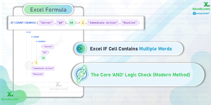
Imagine you are reviewing project status logs in column A. You need to flag any entry that contains both “Server” and “Offline” for immediate action.
=IF(COUNT(SEARCH({word1, word2, ...}, cell)) = number_of_words,
     value_if_true, value_if_false)
This pattern uses SEARCH to find all keywords in the {array} at once, returning their positions. COUNT then tallies only the successful finds (the numbers), and IF compares this count to the total number of words you were looking for.
=IF(COUNT(SEARCH({"Server", "Q4"}, A4)) = 2,
     "Immediate Action", "Routine")
This method is superior for checking 2 or more words. Simply add keywords to the {array} and increase the final count to scale it instantly.
Example 2: The Classic Method for Two Words
This example provides a direct answer for the common query excel if cell contains two words using the traditional IF, AND, and ISNUMBER functions. This method is excellent for understanding the fundamental logic step-by-step and is frequently found in older spreadsheets.
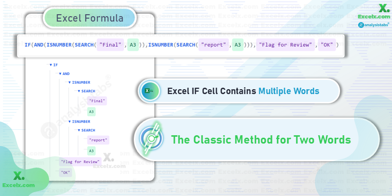
Imagine you’re sorting a product list in column A. You need to flag all items that are described as both “Final” and “report”.
=IF(AND(ISNUMBER(SEARCH("word1", cell)),
        ISNUMBER(SEARCH("word2", cell))),
     value_if_true, value_if_false)
This pattern uses SEARCH to find each word individually. ISNUMBER then confirms if each search was successful (returning a number). AND checks if all individual tests are TRUE before the final IF function gives its result.
=IF(AND(ISNUMBER(SEARCH("Final", A3)),
        ISNUMBER(SEARCH("report", A3))),
     "Flag for Review", "OK")
This formula is clear for two conditions but becomes long and difficult to manage if you need to check for more keywords.
Example 3: Checking Against a Dynamic Keyword Range
This pro-level technique answers the essential query excel if cell contains multiple words mentioned in a Range. Instead of typing keywords into the formula, we reference a list in worksheet cells, making the logic reusable and easy to update.
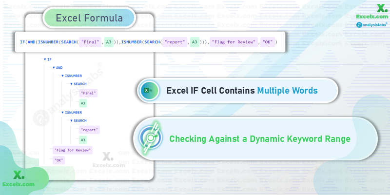
Imagine you are a content manager and need to tag articles in column A based on a list of keywords in C2:C3 that your marketing team frequently changes.
=IF(COUNT(SEARCH(KeywordRange, cell)) = COUNTA(KeywordRange),
     value_if_true, value_if_false)
This formula uses SEARCH to check for all words listed in the KeywordRange. COUNTA automatically counts how many keywords are in your list, making the entire formula dynamic. The $ signs (e.g., $C$2:$C$3) are crucial to lock the reference.
=IF(COUNT(SEARCH($C$2:$C$3, A5)) = COUNTA($C$2:$C$3),
     "Matches All Keywords", "")
This is the most flexible way to manage criteria. To check for more or fewer words, simply edit the list in the keyword range.
Example 4: Combining Text Search with Numeric Conditions
This solution addresses the practical query excel if cell contains multiple conditions by integrating our text search with other logical tests, such as checking a number in an adjacent cell.
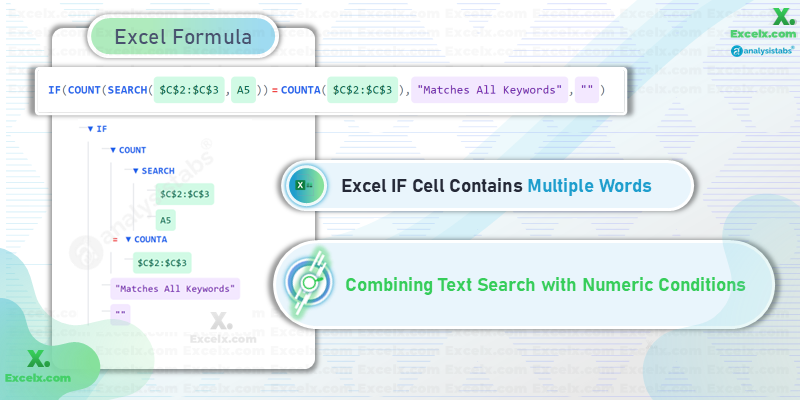
Imagine you are an accounts manager in Bengaluru. You need to flag entries in column A that contain “Urgent” and “Invoice”, but only if the amount in column B is over ₹75,000.
=IF(AND(COUNT(SEARCH({word1, word2}, A2)) = 2,
        B2 > number),
     value_if_true, value_if_false)
This formula uses the AND function as a container. The first condition is our modern COUNT(SEARCH(...)) text check. The second condition is a standard logical test on another cell, like B2 > 75000. Both must be TRUE for the result.
=IF(AND(COUNT(SEARCH({"Urgent","Invoice"}, A2)) = 2,
        B2 > 75000),
     "Escalate for Approval", "Routine")
This pattern is essential for building real-world business logic that depends on multiple factors across different cells.
Example 5: Returning a Specific Value
This directly answers excel if cell contains multiple text then return value. The “value” is simply the value_if_true argument in our IF statement.
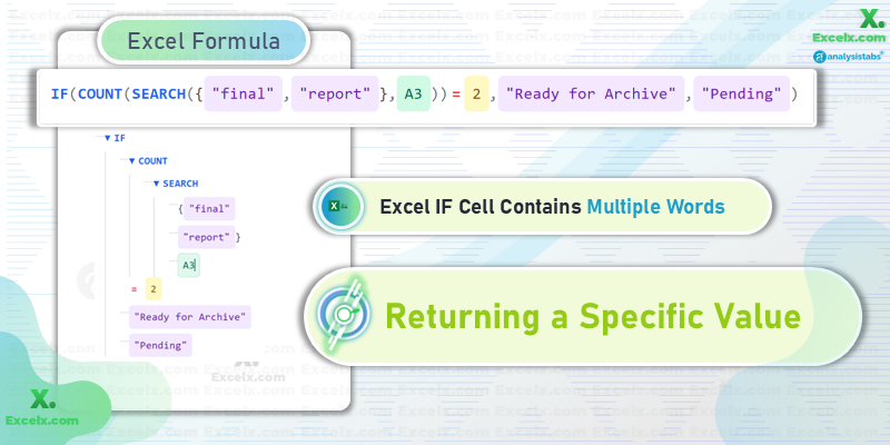
Imagine you are a project manager. If a task in column A contains “Final” AND “report”, you want to mark its status as “Ready for Archive”.
=IF(COUNT(SEARCH({word1, word2}, cell)) = 2,
     "Your Custom Value", "Else Value")
The formula checks for the presence of the keywords. If the logical test is true, the IF function simply returns the text string or value you place in its second argument.
=IF(COUNT(SEARCH({"final","report"}, A3)) = 2,
     "Ready for Archive", "Pending")
This is the most common use case for the IF function: returning a specific, hard-coded label based on a condition.
Example 6: Returning a Corresponding Value from a List
This advanced solution is for if cell contains (multiple text criteria) then return (corresponding text criteria) excel. It uses XLOOKUP to find which word from a list is present and return a corresponding value. (Requires Excel 365/2021).
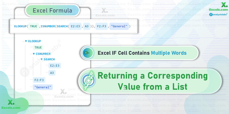
Imagine you have support tickets in column A and a table (in E1:F3) that maps keywords to departments. You want to automatically assign a department.
=XLOOKUP(TRUE, ISNUMBER(SEARCH(KeywordRange, CellToCheck)), ReturnValueRange, "DefaultValue")XLOOKUP searches for TRUE. ISNUMBER(SEARCH(...)) creates an array of TRUE/FALSE values for each keyword. XLOOKUP finds the first TRUE and returns the corresponding item from the ReturnValueRange.
=XLOOKUP(TRUE, ISNUMBER(SEARCH(E2:E3, A3)), F2:F3, "General")This is incredibly powerful for dynamic categorization based on the first keyword found in a priority list.
Example 7: Checking for ANY Word from a List (OR Logic)
This handles the query excel if cell contains multiple text options, where you only need one of the keywords to be present for the condition to be true.
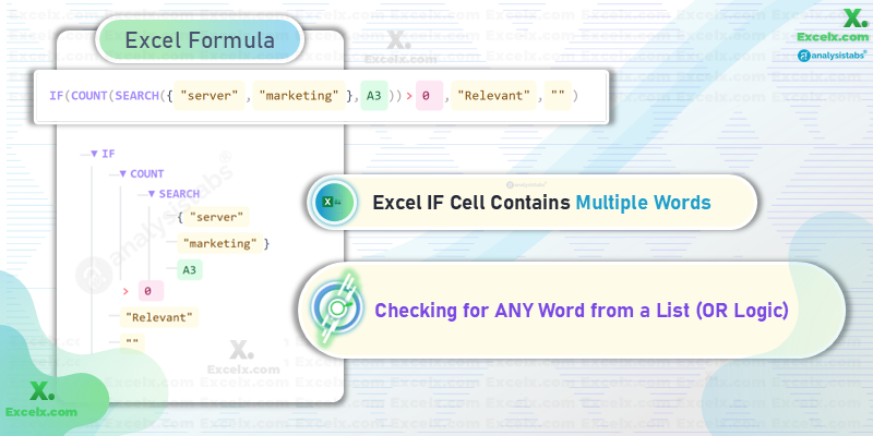
Imagine you want to find any log entry in column A that mentions either “server” OR “marketing” to flag it for review.
=IF(COUNT(SEARCH({word1, word2}, cell)) > 0,
     "At Least One Found", "")
The only change from the core AND logic formula is the comparison operator. Instead of checking if the count equals the total number of words, we just check if it’s > 0.
=IF(COUNT(SEARCH({"server","marketing"}, A3)) > 0,
     "Relevant", "")
If even one word is found, the count will be 1 or more, the condition will be TRUE, and the formula will return the desired result.
Example 8: Counting Rows That Contain Multiple Specific Words
This is the answer for excel count if cell contains multiple specific text. We use SUMPRODUCT, an incredibly powerful array-processing function, to count rows across a range that meet our criteria.
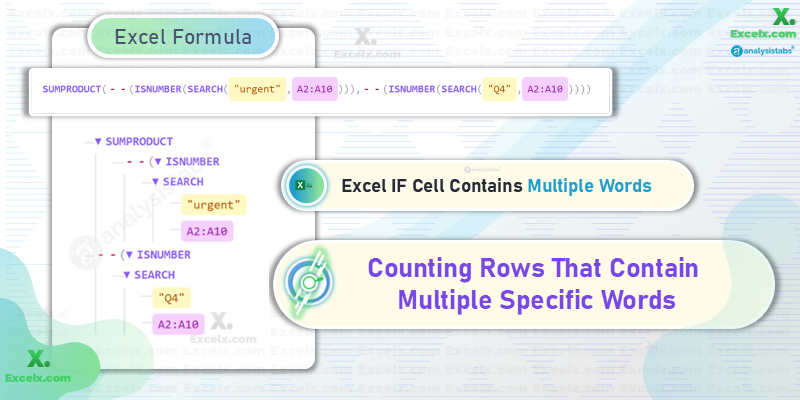
Imagine you want to know the total number of log entries in the range A2:A10 that contain both “urgent” AND “Q4”.
=SUMPRODUCT(--(ISNUMBER(SEARCH(word1, Range))),
             --(ISNUMBER(SEARCH(word2, Range))))
The double-negative -- coerces TRUE/FALSE values into 1s and 0s. SUMPRODUCT multiplies the arrays row by row. A final 1 is only produced if both conditions were TRUE (1 * 1 = 1). It then sums the results.
=SUMPRODUCT(--(ISNUMBER(SEARCH("urgent", A2:A10))),
             --(ISNUMBER(SEARCH("Q4", A2:A10))))
This is the definitive method for counting rows based on complex text criteria within the same cell.
Example 9: Case-Sensitive Check for Multiple Words
This is for when case matters, often related to Excel if cell contains multiple specific text multiple criteria. We simply swap the case-insensitive SEARCH for the case-sensitive FIND.
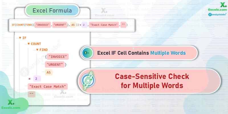
Imagine you need to find log entries in column A that contain both “INVOICE” and “URGENT” in their exact uppercase form.
=IF(COUNT(FIND({Word1, Word2}, cell)) = 2,
     "Case-Sensitive Match", "")
The formula structure is identical to our modern method, but FIND will only return a number if the casing of the text in the cell matches the casing of the keyword exactly.
=IF(COUNT(FIND({"INVOICE", "URGENT"}, A5)) = 2,
     "Exact Case Match", "")
Use this when you need to distinguish between acronyms and regular words (e.g., “IT” vs. “it”).
Example 10: Checking if a Cell Does NOT Contain Certain Words
This handles queries like excel if contains but not. We use the same core logic but check that the count of forbidden words is zero.
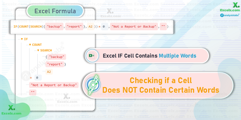
Imagine you want to find all log entries that do not contain the words “backup” or “report”.
=IF(COUNT(SEARCH({forbidden_word1, forbidden_word2}, cell)) = 0,
     "Safe", "Contains Forbidden Word")
The logic is inverted. The formula returns TRUE only if the COUNT of the words you want to exclude is exactly 0.
=IF(COUNT(SEARCH({"backup", "report"}, A2)) = 0,
     "Not a Report or Backup", "")
This is useful for filtering out records or identifying items that have not yet been categorized.
Example 11: Checking for Exact Character Length
For the simple query excel if cell contains 2 characters. This doesn’t check the content, only the total length of the text in the cell.
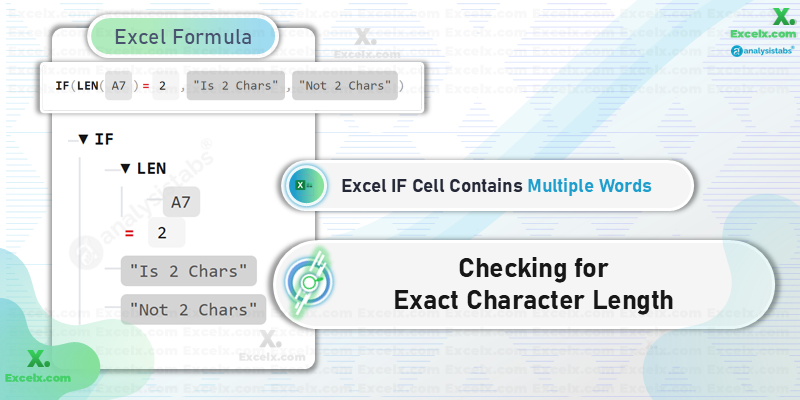
Imagine you need to validate a state code column where entries must be exactly two characters long.
=IF(LEN(CellToCheck) = NumberOfChars,
     "Valid Length", "Invalid Length")
The LEN function simply returns the total number of characters in a cell as an integer, which you can use in a logical test.
=IF(LEN(A7) = 2,
     "Is 2 Chars", "Not 2 Chars")
This is the most efficient way to validate data based on length.
Example 12: Checking for a Specific Number of a Character
This is the best way to solve excel if cell contains two commas or excel if cell contains 2 specific characters.
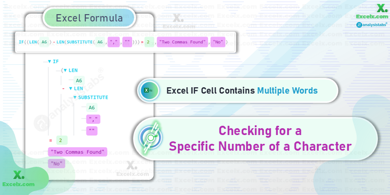
Imagine you are validating a data string in column A that must contain exactly two commas as delimiters.
=IF((LEN(cell) - LEN(SUBSTITUTE(cell, "char", ""))) = Number,
     "Correct Count", "Incorrect Count")
This clever trick measures the cell’s length before and after the SUBSTITUTE function removes all instances of the character in question. The difference in length is the number of occurrences.
=IF((LEN(A6) - LEN(SUBSTITUTE(A6, ",", ""))) = 2,
     "Two Commas Found", "No")
This is a highly efficient way to count any single character within a text string.
Example 13: Checking if a Cell *Starts With* One Word and *Contains* Another
This handles the specific excel if starts with and contains query by combining two different search techniques.
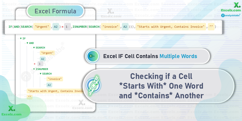
Imagine you need to identify log entries in column A that must start with the word “Urgent” and also contain the word “invoice” anywhere in the text.
=IF(AND(SEARCH(start_word, cell) = 1,
        ISNUMBER(SEARCH(contains_word, cell))),
     "Meets Criteria", "")
This formula uses the classic AND structure. The first part, SEARCH(start_word, cell) = 1, explicitly checks if the first keyword’s starting position is the very first character.
=IF(AND(SEARCH("Urgent", A2) = 1,
        ISNUMBER(SEARCH("invoice", A2))),
     "Starts with Urgent, Contains Invoice", "")
This demonstrates how to combine positional logic with general containment logic.
Example 14: Combining AND & OR Logic
For complex queries like excel if contains x and y or z. Here we check for (“final” AND “report”) OR (“urgent”).
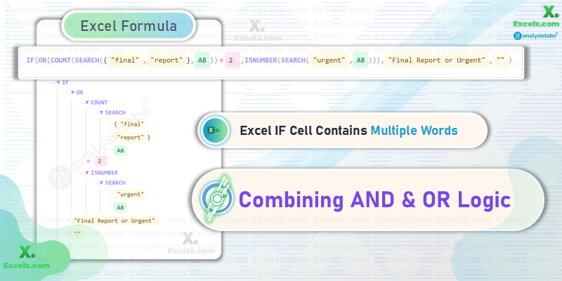
Imagine you need to flag any log entry that is either an urgent task of any kind, or specifically a final report.
=IF(OR(COUNT(SEARCH({word_A, word_B}, cell)) = 2,
        ISNUMBER(SEARCH(word_C, cell))),
     "Condition Met", "")
The OR function acts as the main container. It returns TRUE if either of its conditions are met: the first is our multi-word AND check, and the second is a single-word check.
=IF(OR(COUNT(SEARCH({"final","report"}, A8)) = 2,
        ISNUMBER(SEARCH("urgent", A8))),
     "Final Report or Urgent", "")
This nested structure is key to building complex business rules in Excel.
Example 15: Using `IFERROR` as an Alternative
For the query excel iferror with search, this method can create logical tests by converting errors to 0 and successful finds to a positive number.

Imagine you want to check for “final” and “report” in column A using a multiplication-based logic.
=IF(IFERROR(SEARCH(word1, cell), 0) * IFERROR(SEARCH(word2, cell), 0) > 0,
     "Both Found", "One or more missing")
If a SEARCH fails, IFERROR returns 0. If it succeeds, it returns a number greater than 0. By multiplying the results, the final product will only be greater than zero if *both* searches were successful.
=IF(IFERROR(SEARCH("final", A8), 0) * IFERROR(SEARCH("report", A8), 0) > 0,
     "Match Found", "No Match")
While clever, the COUNT(SEARCH(...)) method is generally more readable and scalable.
Example 16: Filtering a List Based on Multiple Contained Words
The solution for excel filter if cell contains multiple text using modern Excel’s powerful FILTER function.
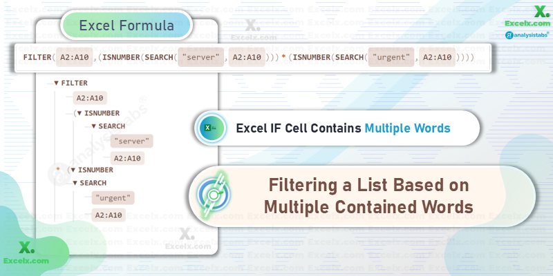
Imagine you want to extract a list of all log entries from A2:A10 that contain both “server” AND “urgent”.
=FILTER(RangeToFilter,
        (ISNUMBER(SEARCH(word1, RangeToCheck))) * (ISNUMBER(SEARCH(word2, RangeToCheck))))
The FILTER function spills a list of results that meet the criteria. The asterisk * acts as an AND operator in array logic, ensuring both conditions are met for a row to be included.
=FILTER(A2:A10,
        (ISNUMBER(SEARCH("server", A2:A10))) * (ISNUMBER(SEARCH("urgent", A2:A10))))
This is the most direct way to extract matching data in Microsoft 365.
Example 17: Matching Multiple Specific Phrases
This addresses the query excel if cell contains multiple specific text when dealing with multi-word phrases instead of single words.
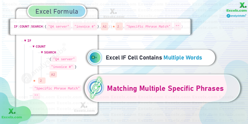
Imagine you need to identify descriptions in column A that contain the exact phrase “Q4 server” AND the exact phrase “invoice #”.
=IF(COUNT(SEARCH({"phrase 1", "phrase 2"}, cell)) = 2,
     "Match", "No Match")
The modern method works perfectly for phrases just as it does for single words. Simply include the entire phrase in quotes within the array constant.
=IF(COUNT(SEARCH({"Q4 server", "invoice #"}, A2)) = 2,
     "Specific Phrase Match", "")
This confirms the power and flexibility of the COUNT/SEARCH pattern.
Example 18: Checking for Text Between Delimiters
This is an advanced technique for when you need to know if text exists between two specific characters, like parentheses or brackets.
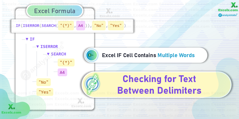
Imagine you want to flag any log entry in column A that has text inside parentheses, like “(urgent)”.
=IF(ISERROR(SEARCH("(*)", cell)), "No Parentheses", "Contains Parentheses")This uses SEARCH with wildcards. * matches any number of characters. The formula looks for an opening parenthesis, followed by any text, followed by a closing parenthesis.
=IF(ISERROR(SEARCH("(*)", A4)), "No", "Yes")This is a quick way to check for patterns in your data, not just specific words.
Example 19: The Google Sheets `REGEXMATCH` Solution
The definitive solution for if cell contains (multiple text criteria) ... google sheets, using the powerful regular expression function.
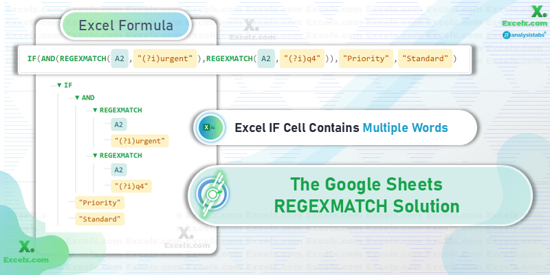
Imagine you are in Google Sheets and need to check if cell A2 contains both “urgent” and “q4”.
=IF(AND(REGEXMATCH(A2, "(?i)word1"), REGEXMATCH(A2, "(?i)word2")), "Yes", "No")REGEXMATCH is Google Sheets’ tool for advanced text pattern matching. The (?i) is a flag within the expression that makes the search case-insensitive. We use AND to ensure two separate tests both return TRUE.
=IF(AND(REGEXMATCH(A2, "(?i)urgent"), REGEXMATCH(A2, "(?i)q4")), "Priority", "Standard")Regular expressions offer immense power for complex text matching beyond what is easily achievable in Excel without VBA.
Example 20: The Ultimate Dynamic, Case-Sensitive Pattern
This combines multiple advanced techniques into a single, robust formula for the most demanding criteria, often related to Excel if cell contains multiple specific text formula.
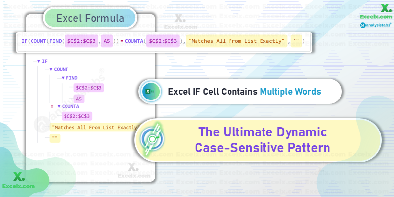
Imagine you must check if a log entry contains all keywords from a dynamic list (in C2:C3), and the match must be case-sensitive.
=IF(COUNT(FIND(KeywordRange, cell)) = COUNTA(KeywordRange),
     "All Found (Case-Sensitive)", "")
This formula is the ultimate combination of best practices: it’s case-sensitive (FIND), it checks for all keywords (COUNT), and it is fully dynamic by referencing a cell range (KeywordRange) and automatically counting the criteria (COUNTA).
=IF(COUNT(FIND($C$2:$C$3, A5)) = COUNTA($C$2:$C$3),
     "Matches All From List Exactly", "")
Mastering this pattern means you can build highly specific, maintainable, and powerful logical tests for any text-based data.
Automation Corner: VBA & Office Scripts
When you need to perform the same checks repeatedly or on very large datasets, manual formulas can become inefficient. Automation using VBA (for desktop Excel) or Office Scripts (for Excel on the Web) can save you hours of work. Here are practical examples for both platforms.
VBA Examples for Desktop Excel
VBA (Visual Basic for Applications) is the long-standing automation tool built into desktop versions of Excel. It’s incredibly powerful for creating custom functions and automating complex workflows.
VBA Example 1: A Reusable Custom Function (‘ContainsAll’)
Instead of typing a long formula every time, you can create your own worksheet function. This makes your formulas shorter, easier to read, and less prone to errors.
How to Install:
- Open your Excel file and press
Alt + F11to open the VBA Editor. - In the menu, click
Insert > Moduleto create a new code module. - Copy and paste the code below into the white text area.
- Close the VBA Editor and return to Excel. Your function is ready to use!
' VBA Code for a Custom Worksheet Function
' Created on: August 11, 2025 in Bengaluru, Karnataka
Function ContainsAll(checkCell As Range, ParamArray keywords() As Variant) As Boolean
    ' This function checks if a single cell contains ALL of the specified keywords.
    ' It is case-insensitive.

    Dim keyword As Variant
    Dim cellContent As String

    ' Ensure we only work with the first cell if a range is passed
    cellContent = LCase(checkCell.Cells(1, 1).Value)

    ' Loop through each keyword provided in the function arguments
    For Each keyword In keywords
        ' If any keyword is not found, immediately exit and return FALSE
        If InStr(1, cellContent, LCase(keyword)) = 0 Then
            ContainsAll = False
            Exit Function
        End If
    Next keyword

    ' If the loop completes, it means all keywords were found.
    ContainsAll = True
End Function
How to Use in Excel:
Now, you can use this function directly in a cell just like any built-in function. It’s much cleaner than the original formula.
=IF(ContainsAll(A2, "urgent", "q4", "invoice"), "High Priority", "Standard")VBA Example 2: Find and Highlight Matching Rows
This is a more powerful example that automates a complete task. This subroutine will loop through all your data, find the rows that contain all your specified keywords, and highlight them in yellow for immediate visual analysis.
How to Use:
- Install the code in a VBA Module using the same steps as above.
- Return to your Excel sheet.
- Press
Alt + F8to open the Macro dialog box. - Select “HighlightMatchingRows” and click “Run”.
- A prompt will ask you to enter your keywords, separated by commas.
' VBA Subroutine to find and highlight rows
Sub HighlightMatchingRows()
    Dim ws As Worksheet
    Dim searchRange As Range
    Dim cell As Range
    Dim keywordsInput As String
    Dim keywords() As String
    Dim keyword As Variant
    Dim allFound As Boolean
    Dim lastRow As Long

    ' Set the worksheet you are working on
    Set ws = ActiveSheet

    ' Determine the last row with data in Column A
    lastRow = ws.Cells(ws.Rows.Count, "A").End(xlUp).Row
    If lastRow < 2 Then Exit Sub ' Exit if no data

    ' Define the range to search (e.g., A2 to the last row)
    Set searchRange = ws.Range("A2:A" & lastRow)

    ' Clear previous highlighting
    ws.Rows("2:" & lastRow).Interior.Color = xlNone

    ' Prompt the user for keywords
    keywordsInput = InputBox("Enter keywords separated by a comma (e.g., urgent,q4,server)", "Keyword Search")
    If keywordsInput = "" Then Exit Sub ' Exit if user cancels

    ' Split the user's input into an array of keywords
    keywords = Split(keywordsInput, ",")

    ' Loop through each cell in the defined range
    For Each cell In searchRange
        allFound = True ' Assume all are found until proven otherwise

        For Each keyword In keywords
            ' Check if a keyword is NOT in the cell (case-insensitive)
            If InStr(1, LCase(cell.Value), Trim(LCase(keyword))) = 0 Then
                allFound = False ' Mark as not found
                Exit For ' No need to check other keywords for this cell
            End If
        Next keyword

        ' If after all checks, all keywords were found, highlight the row
        If allFound Then
            cell.EntireRow.Interior.Color = vbYellow
        End If
    Next cell

    MsgBox "Highlighting complete."
End Sub
Modern Automation: Office Scripts for Excel on the Web
Office Scripts are the modern, cloud-first successor to VBA. They use TypeScript (a superset of JavaScript) and are designed for secure, shareable automation in Excel for the Web. They can also be integrated with Power Automate to create powerful, cross-application workflows.
Office Script Example: Find and Tag Matching Rows
This script performs a similar task to the VBA subroutine: it reads through your data, finds rows containing a set of keywords, and writes a status in an adjacent column. This is perfect for collaborative, cloud-based workflows.
How to Use:
- In Excel on the Web, go to the Automate tab.
- Click New Script to open the Code Editor.
- Copy and paste the entire code block below into the editor, replacing any existing code.
- Click Save script and give it a name like “Tag Matching Rows”.
- Click Run to execute the script on your active worksheet.
// Office Script for Excel on the Web
// Created on: August 11, 2025 in Bengaluru, India

function main(workbook: ExcelScript.Workbook) {
  // Get the active worksheet
  const selectedSheet = workbook.getActiveWorksheet();

  // --- Configuration ---
  const keywordsToFind: string[] = ["urgent", "server"];
  const searchColumnIndex: number = 0; // Column A (0-indexed)
  const tagColumnIndex: number = 3;    // Column D (0-indexed)
  const tagText: string = "Flagged for Review";
  // -------------------

  // Get the range of data in the worksheet, excluding the header row
  const dataRange = selectedSheet.getUsedRange();
  if (dataRange.getRowCount() <= 1) {
    console.log("No data to process.");
    return;
  }
  const dataValues = dataRange.getValues();

  console.log(`Checking ${dataRange.getRowCount() - 1} rows for keywords: ${keywordsToFind.join(', ')}`);

  // Loop through each row of the data (starting from the second row)
  for (let i = 1; i < dataValues.length; i++) {
    const row = dataValues[i];
    const cellValue = (row[searchColumnIndex] as string).toLowerCase();
    let allKeywordsFound = true;

    // Check if the cell content is valid
    if (cellValue) {
      // Check for the presence of each keyword
      for (const keyword of keywordsToFind) {
        if (!cellValue.includes(keyword.toLowerCase())) {
          allKeywordsFound = false;
          break; // Stop checking this row if a keyword is missing
        }
      }

      // If all keywords were found, write the tag in the specified column
      if (allKeywordsFound) {
        selectedSheet.getCell(i, tagColumnIndex).setValue(tagText);
        console.log(`Row ${i + 1}: Match found. Tagged.`);
      }
    }
  }
  console.log("Script finished.");
}
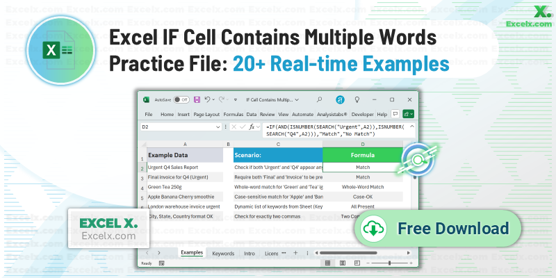
Download practice workbook
To help you master the techniques shown above, we’ve prepared a ready-to-use Excel practice file. It contains realistic text entries alongside six live “IF Cell Contains Multiple Words” formulas, including classic AND + SEARCH, whole-word matching, case-sensitive checks, dynamic list lookups, comma-count validation, and scalable keyword tests. Each example includes the data, formula, and a clear description so you can see exactly how the logic works. No VBA is required, and the file is fully compatible with Microsoft 365 and Excel 2021+.
Frequently Asked Questions
Can I use AND logic to search for more than two words in a cell?
Yes. You can expand the formula by adding more ISNUMBER(SEARCH("word",cell)) tests inside the AND function. For example, to check for “Green”, “Tea”, and “Organic” all in one cell:
=IF(AND(ISNUMBER(SEARCH("Green",A2)),
        ISNUMBER(SEARCH("Tea",A2)),
        ISNUMBER(SEARCH("Organic",A2))),
    "Match","No Match")
How do I make the formula case sensitive?
Replace SEARCH with FIND. Unlike SEARCH, FIND distinguishes between uppercase and lowercase, so “Tea” will not match “tea”. Example:
=IF(AND(ISNUMBER(FIND("Green",A2)),
        ISNUMBER(FIND("Tea",A2))),
    "Match","No Match")
What if one of the words might appear multiple times?
The formula still works because SEARCH and FIND only need to find the first occurrence. If a word appears multiple times, the function still returns a number and the AND logic remains valid.
How can I search for words from a named range instead of typing them in?
Store your keywords in a named range (e.g., Keywords) and use a dynamic COUNT+SEARCH approach:
=IF(SUM(--ISNUMBER(SEARCH(Keywords,A2)))=ROWS(Keywords),
    "Match","No Match")
Can I return something other than “Match” or “No Match”?
Yes. Replace the last two arguments of the IF function with your preferred output values. For example:
=IF(AND(ISNUMBER(SEARCH("Green",A2)),
        ISNUMBER(SEARCH("Tea",A2))),
    "Include in Report","Skip")
Will this work on numbers as well as text?
Yes. SEARCH and FIND can also locate numbers stored as text. For actual numeric comparisons, replace the SEARCH logic with your own conditions, such as A2>100 or AND(A2>100,B2<50).
What’s the best way to avoid #VALUE! errors?
Always wrap SEARCH or FIND inside ISNUMBER, as this converts errors into FALSE values. Without this, missing words will trigger #VALUE! errors that break your formula.
Can I use wildcards in the search terms?
SEARCH supports wildcards when combined with other functions like COUNTIF, but within SEARCH itself, wildcards aren’t necessary because it matches partial text. For example, searching for “Tea” will match “Teapot” as well.