Very often we reference the data of a Cell in another Cell in Excel. We can use equals to sign (=) then enter the cell address to display Cell contents in another Cell. Let us see how to display cell contents in another cell in Excel in this topic.
Referencing the Cell Contents in Another Cell
Double click on any Cell in Excel Sheet to make the Cell editable. Then enter the equals to sign (=) and enter the address of Cell which you wants to refer. You can refer a single Cell or a Range using this approach. Here are the examples on referencing the content of a Cell and displaying in another cell in Excel. Let us see the detailed examples on referencing the cells in the following scenarios.
It is very important to know the types of cell references we can use while referencing the cells in Excel. There are two types of references in Excel, Relative and Absolute References.
Referencing a specific Cell
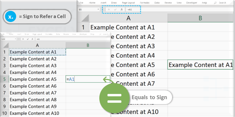
We can enter ‘=’ sign and specify the cell address in any cell in the Excel Sheet. For example, you can enter ‘=A1’ at Range B1 to refer the Cell content of A1 in B1, you can enter ‘=AB25’ at C5 to refer the content of range AB25 in Range C5.
Begin with = Sign to Refer a Cell
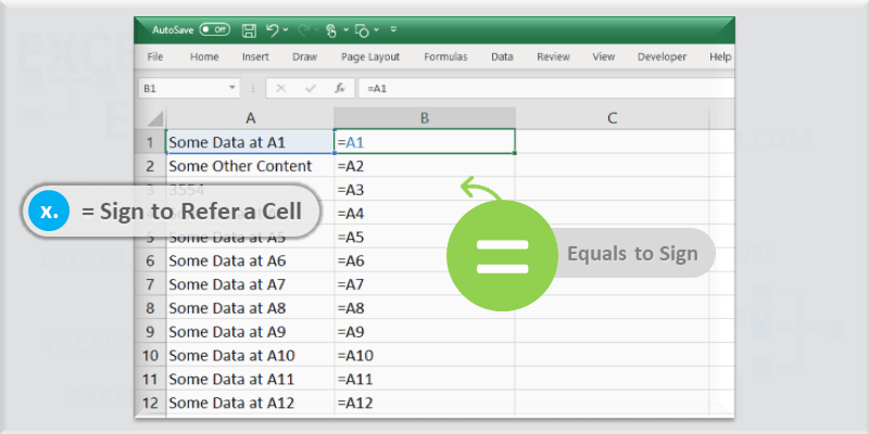
Equals to sign (=) is used to refer Cell in Another Cell
Referencing a Cell in Excel
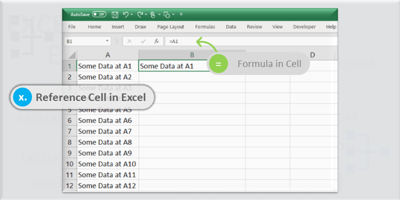
Formula Bar Showing a Cell Content in another Cell
Displaying Cell Content in Excel
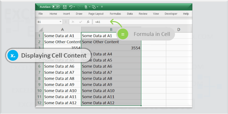
Showing a Cell Content in another Cell in Excel
Fill down the Formula in Excel
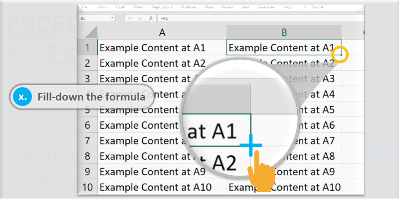
Double Click or Drag down with mouse
Relative Reference in Excel
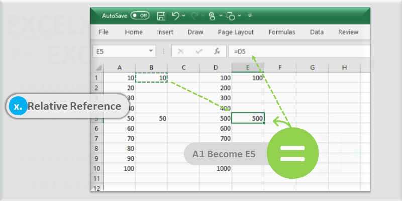
Relative reference is used to change the Cell Column or Row relatively while copying the cells with formula to another range. Row number and Column Names will changes relatively when we use relative cell reference.
For example, when you have =A1 reference in Cell B1, it will change to A2 while copying down to the next row (i.e; A2), it will chnage to B1 when copying to the next Column (i.e; C1). The change in number of columns and rows depending to the relative number of columns and rows which you are pasting the cells.
For example, if you copy the same ‘=A1’ reference in Cell B1, it will change to A5 when you paste at cell B1, it will become D5 when you paste in E5.
Relative Reference in Excel
Do not use $ to create Relative Cell References
Relative Reference – Formula in Excel

Cell Formula will changes relatively in Relative Reference
Display Text From Another cell in Excel
We can display the text of another cell using Excel Formula. We can use ‘=’ assignment operator to pull the text from another cell in Excel. You can show text from another cell in Excel using the formula below.
For example, the following formula will get the text from Cell D5 and display in Cell B2.
=D5
You can enter =D5 in Range B2. You can use ‘$’ symbol to make the cell reference as absolute (=$D$5).
Display Value From Another cell in Excel
We can display the Value of another cell using Excel Formula. We can use ‘=’ assignment operator to pull the value of another cell in Excel.
For example, the following formula will get the value from Cell C6 and display in Cell A3.
=C6
You can enter =C6 in Range A3. You can use ‘$’ symbol to make the cell reference as absolute (=$C$6).
Referencing a Range (multiple cells)
We can refer multiple Cells in Excel using Excel Formula. We can get the cell contents and display in a cell or refer the range to perform calculations.
Getting Values From Multiple Cells in Excel
Often we refer the multiple cells in put into once Cell. We can refer the multiple Cells and Ranges in Excel to combine the text or to perform the calculations.
Getting Text from Multiple Cells
The following formula will refer the text from multiple cells and combine them to display in one Cell. This will get the contents form Cell E2 and F2 and display the combined text in another Cell.
=E2&F2
Combine Text of Multiple Cells:
We can use & operator to concatenate the text from multiple cells. We can provide a space or – to separate the text to form multiple words. The following Example shows you how to get the data from multiple cells and display the combined text in one cell.
=E2&" " &F2
Getting Values from Multiple Cells:
Sometimes, we need to pull the values of another cell and perform some calculations in a cell. For example, We have Cost and Quantity values in two different cells (B2,C2) and we can find the total cost in another Cell (A2).
=B2*C2
Combining Values of Multiple Cells:
We can also combine the numerical data of multiple cells using & operator. We can concatenate both Text and numerical data and display in required Cell. The following example shows you how to get the different formats of data from multiple cells and display the combined information in a cell.
=" Total Cost is " &B2*C2
Referring Data from a Range of Cells
The following example shows you referring a range and perform mathematical calculations. It will reference Range D1 to E5 and put the Sum of the data in Range A1
=SUM(D1:E5)
Referencing Cells from another Sheet
Referencing the Cells from one sheet is very easy in Excel. We need to pass the Sheet Name in the Formula followed by ‘!’ symbol. Exclamation symbol is used to refer the Worksheet in the Excel Formula.
The following example will refer the Cell content form another worksheet (Data) and display in a Cell.
=Data!A1
We need to put the sheet name between single quotes when the Sheet name is having multiple words. For example the following formula will refer the Cell form another sheet named with multiple words (Data Sheet)
='Data Sheet'!A1
Referencing and Concatenating Cells
We can concatenate the Cells using Concatenate operator or using CONCATENATE Function in Excel. Let us see the both the methods to concatenate Cells in Excel.
Using Concatenate Operator: You can refer the cells using the Cell address and use the & (ampersand) operator to concatenate the Cells. For example, the following formula will concatenate cells (D1 and E1).
=D1&E1

'OR

=D1&" "&E1
Using CONCATENATE Function: We can use the Excel Function to refer and concatenate multiple cells and ranges in Excel. You use the , (comma) t0 specify the reference of each Cell in the formula.
=CONCATENATE(D1,E1)
Referencing a Named Range
We can refer the Named Ranges in Excel using Formula. Name of Range should follow the = operator to refer a named range in Excel. The following Formula refer the named range called ‘TotalSales’.
=TotalSales
The will display the Cell value which is named as ‘TotalSales’.
The following examples shows you, how to refer the range of cells in Excel. The Range (‘Sales Column’) is referred in SUM function to return the total value of ‘Sales Column’ Named Range.
=SUM('Sales Column')
Showing Cell values on a Shape
Follow the below instructions to display the cell contents on a Shape.
- Select the Shape
- Click on the Formula bar
- Enter the = (assignment) operator
- And put required Cell Address (For example: =$A$3)
Showing Cell value in Chart Title
Follow the below instructions to display the cell contents in Chart Title.
- Select the Chart which you want to display the Cell Value
- Go to ‘Chart Design’ Tab in the Ribbon
- And Show the Chart Title from Chart Elements
- Click on Chart Title of the Selected Chart
- Click on the Formula bar
- Enter the = (assignment) operator
- And put required Cell Address (for example: =Sheet2!$K$8)
Working with Formulas as Text
Sometimes you may want to see the actual formula instead of its resulting value. Excel’s FORMULATEXT function lets you display the formula from another cell as plain text. This is especially useful when you need to audit, share, or document your formulas.
- Example:
If cell B1 contains a formula (=SUM(A1:A10)), enter in cell C1:=FORMULATEXT(B1)
This displays the exact formula (=SUM(A1:A10)) used in B1.
Note: If Excel shows the formula as text instead of its result, check that the cell’s format is set to General and that no leading apostrophes are present.
Combining Text and Formulas
Creating dynamic messages or reports in Excel often requires you to mix cell values (or formulas) with static text.
- Using the Ampersand (&) Operator:
Combine text with cell references easily.
Example:="Total Cost is " & B2 * C2
This joins the text with the calculated result of multiplying B2 by C2.
- Using the CONCATENATE Function:
Alternatively, you can use:
Example:=CONCATENATE("Total: ", B2)Both methods allow you to build formulas that include both text and cell data.
These techniques answer queries such as “excel formula & text” and “excel formula to insert text from another cell.”
Advanced Techniques: Referencing Across Worksheets and Named Ranges
For larger or multi-sheet workbooks, linking cells from different worksheets or using named ranges can significantly boost efficiency.
- Referencing Cells from Another Sheet:
Use the sheet name followed by an exclamation mark.
Example:=Sheet2!A1
If the sheet name contains spaces, enclose it in single quotes:
='Data Sheet'!A1
- Using Named Ranges:
Assign a name to a cell or range and refer to it directly.
Example:=TotalSales
This method simplifies complex formulas and enhances clarity.
These techniques are ideal for queries like “excel reference cell in another sheet” and “excel pull data from another worksheet.”
Auto-Filling and Linking Cells Based on Another Cell’s Value
Excel allows you to auto-populate cells and create dynamic links between them—ensuring that changes in one cell automatically update the linked cells.
- Auto-Fill Using the Fill Handle:
Write a formula (e.g., =A1) and drag the fill handle to copy it. Excel automatically adjusts relative references. - Linking Cells for Dynamic Updates:
When one cell’s value changes, any cell linked with a simple reference (or formula) updates instantly.
This technique answers questions like “excel typing in one cell appears in another” and “how to pull data from one cell to another in excel.”
Troubleshooting Common Errors
Even experienced Excel users sometimes encounter issues. Here are some common errors and their solutions:
- #REF! Error:
Indicates an invalid cell reference (for example, if a referenced cell was deleted).
Solution: Verify and update the reference. - Formulas Displaying as Text:
Occurs if the cell is formatted as Text or if a leading apostrophe is used.
Solution: Change the cell format to General or remove the apostrophe. - Incorrect Relative References:
Copying formulas may inadvertently change the intended cell references.
Solution: Use absolute references (e.g., =$A$1) when necessary.
These tips cover issues mentioned in queries like “excel formula showing as text” and “how to copy value from one cell to another in excel using formula.”
Frequently Asked Questions (FAQs)
Q1: How can I display a cell’s formula as text?
A: Use the FORMULATEXT function (e.g., =FORMULATEXT(B1)) to reveal the formula in a cell.
Q2: How do I reference text from one cell in a formula?
A: Simply use a cell reference (e.g., =A1). Excel will display the text contained in that cell.
Q3: How do I combine static text with cell values?
A: Use the ampersand (&) operator or the CONCATENATE function. For example, =”Total: ” & B2 combines text with the value from B2.
Q4: What is the proper way to reference cells from another worksheet?
A: Use the syntax =SheetName!A1 or, if the sheet name has spaces, =’Sheet Name’!A1.
Q5: Why might my Excel formula display as plain text instead of calculating?
A: This often happens if the cell is formatted as Text or if there is a preceding apostrophe. Changing the format to General usually fixes the issue.
Q6: How do I ensure that a reference stays constant when copying a formula?
A: Use absolute references by adding dollar signs (e.g., =$A$1).
Q7: How can I auto-fill cells based on another cell’s content?
A: Use Excel’s fill handle to drag and copy formulas, ensuring that relative references update appropriately.
Q8: How do I reference a named range?
A: Once defined, simply type the name (e.g., =TotalSales) in your formula to refer to that range.
These FAQs address many common queries, such as “excel show formula as text in another cell,” “excel reference text in another cell in formula,” and “how to display cell formulas in excel.”
Conclusion & Key Takeaways
Mastering how to display and reference cell contents, formulas, and text in Excel is essential for creating efficient, dynamic spreadsheets. By:
- Using FORMULATEXT to reveal formulas,
- Combining text with cell values for dynamic reporting,
- Linking cells across worksheets,
- And applying best practices for troubleshooting and organization,
you’ll be better equipped to build robust and error-resistant workbooks. Experiment with these techniques to streamline your workflow and boost your Excel efficiency.

I’d like to learn a formula that will identify a character, for example “_”, and return the contents of the next cell. The results are pulled from a data sheet and compiled into a list/column.
For example, if d:d contains “_” show contents of f:f
Any help would nmbe appreciate!
How would you format a cell to show the content of another selected cell in the same sheet?
I’m thinking of a text search function that actively translates the content of a selected cell in a column, maybe using the Googletranslate function, but I’m currently stuck on the first part of getting the content.
Hello!
I have a cell that contains the address of another cell. How can I get the value of this cell?
Let’s say your Cell B1 contains the address of Cell A1, and you want to get the value of Cell A1?
how to pupulate sheet 1 A field data based on sheet 2 table – example Sheet 1 having country, name, sheet 2 is having country name with values in it
i want to fill Sheet 1 A field data referring sheet 2 table
Hi, You can use the VLookUp to display the values from another Sheet. Please see the below formula:
Hi, is there a way to show the value of A1 to B1 but the formula should not be in B1? Also B1 should be editable if the value of A1 is false? Thanks
You can use VBA code as shown below:
Private Sub Worksheet_Change(ByVal Target As Range)
If Target.Address = Range("A1").Address And Range("A1") <> False Then
Range("B1") = Range("A1")
End If
End Sub
You can call this macro in Worksheet Module, it will enter the A1 value into B1 if A1<> False. so that you can edit and enter your own value in B1 when A1 is False.
Hope this helps!
i need a formula that having minimum and maximum condition and get result as minimum or maximum cell adjacent cell value
Hi! In my Excel 2021 I can use reference to range in one cell to see data from all cells in range ( Example: = A2:A7). These data i can copy and paste as Values in other location for usage.
However in other PC I see only data from one cell. Is it specific for Excel version or Excel Options?
how do I display contents of a cell in a sheet of one excel file to a cell of a sheet in 2nd excel file
Here is an Example to display content from Range A1 form Sheet1 in SourceWorkbook1:
Hi! How can I “print” values, let’s say in cell “A1”, and than storage that value in cell “B1” erasing the value in cell “A1”? I didn’t find anything about this automation.
You can use VBA, please describe your requirement clearly.
Thanks
PNRao!
Hello! Awesome site/info here. Well done.
Quick question- is there a formula that can display the NOTE embedded in one cell, as text in another cell? For example, if I have a budget note in B12, can i display the note in that cell in B13 as text?
Thanks.
It is not possible with Excel Formula, you can use the below user defined VBA function to display the notes of a range in the cell.
'Place this in you VBA Code module
Function MyNote(ByVal rng As Range) As String
    On Error GoTo skipThis
    MyNote = rng.Comment.Text
skipThis:
End Function
Now you use this formula in B13=MyNote(B12)
Hope this helps!
Thanks
PNRao
I have performed a lookup to establish the maximum record for a set of criteria, once i have that result, i want to display text from another column that is matched to the maximum record, so for example a list of apples oranges pears and bananas. each has a number of sales, I can find the maximum by using =MAXIFS which gives me the maximum value based on the criteria (i.e apples, etc), but I would like to display another part of the row which is not referenced in the MAXIFS formula, it may be 10 rows to the right or 6 rows to the left of the MAXIFS result number
Hello! Quick question- is there a way to insert the reference to a cell (a number) into the contents of another cell? For example, if I have a long description in cell A1 containing a number that is in cell A5 and I would like the long description of cell A1 to include a reference to cell A5 (which changes continuously).
Thanks for your attention and apologize for my terrific english.
Best regards.
Hello,
I would like to automate the below.
=’Load case 1′!$A$6
I want to replace ‘Load case 1’ with the name of the rest sheets. To populate the rest of the cells with ‘Load case 2’ , ‘Load case 3’ etc, which are the name of autogenerated sheets from a program. I will always want to get back the A6 cell from each sheet.
Thanks
=INDIRECT("'" & A1 & "'!$A$6")Explanation:
A1: This cell contains the sheet name (e.g., “Load case 1”).
“‘ and ‘!”: These parts are used to format the sheet name correctly in the INDIRECT function, ensuring it’s treated as a valid reference.
$A$6: This is the cell from which you want to fetch the data (you can adjust this if you want a different cell).
Or use the below VBA code to automate this process:
Sub PopulateCellsWithSheetData()
    Dim ws As Worksheet
    Dim i As Integer
    Dim sheetName As String
    Dim formula As String

    ' Loop through all sheets in the workbook
    For Each ws In ThisWorkbook.Sheets
        ' Skip sheets that do not match the pattern "Load case #"
        If InStr(ws.Name, "Load case") > 0 Then
            ' Construct the formula for A6 in each sheet
            formula = "=''" & ws.Name & "''!$A$6"
            ' Find the next empty row in the column you want to place the formula
            i = Cells(Rows.Count, 1).End(xlUp).Row + 1
            ' Place the formula in the next row
            Cells(i, 1).Formula = formula
        End If
    Next ws
End Sub
Thanks
PNRao!