Have you ever scrolled down a massive Excel spreadsheet, only to realize you’ve completely forgotten what the data in “Column J” actually represents? You have to scroll all the way back up to check the header, scroll back down, find your spot, and repeat the process five minutes later.
It is annoying, it breaks your flow, and it is completely unnecessary.
The solution is the Freeze Panes feature (often called “fixing panes”). Whether you need to lock the header row, freeze multiple columns, or lock rows and columns horizontally and vertically, this guide covers every method.
Key Highlights
- Freeze Top Row: Keeps the very first row visible while scrolling down.
- Freeze First Column: Keeps Column A visible while scrolling to the right.
- Freeze Custom Selection: Lock specific rows (like the top 2) or multiple columns based on your needs.
- Freeze Panes Shortcut:
Alt+W+F+F(Custom Freeze). - Mobile App Support: Learn how to turn off or on freeze panes in Excel Mobile to fix scrolling issues.
Method 1: How to Freeze the Top Row (Header Row)
This is the feature 90% of users need. You have a simple header in Row 1, and you want it to stick to the top of your screen.
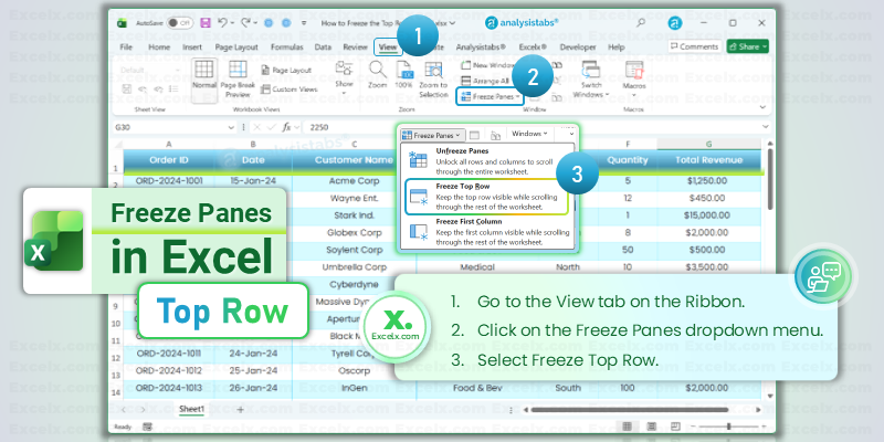
- Open your Excel spreadsheet.
- Go to the View tab on the Ribbon.
- Click on the Freeze Panes dropdown menu.
- Select Freeze Top Row.
How to tell if it worked:
Scroll down. You will notice a thin, solid line appear below Row 1. As you scroll past Row 20, 50, or 100, Row 1 will stay locked at the top.
Method 2: How to Freeze the First Column
If you have a wide dataset (scrolling horizontally), you might lose track of the “Customer Name” or “Order ID” in Column A. Here is how to lock it.
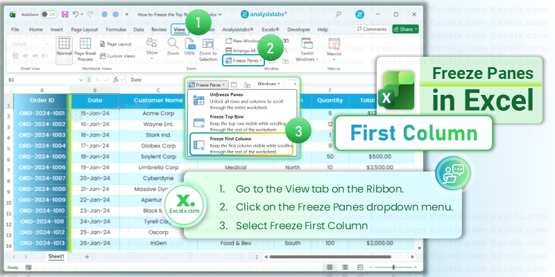
- Go to the View tab.
- Click Freeze Panes.
- Select Freeze First Column.
Method 3: How to Freeze Multiple Rows or Columns (Custom Freeze)
The standard buttons only freeze one row or one column. But what if you need to freeze the top 2 rows (e.g., Title + Header) or freeze selected columns?
You must use the custom Freeze Panes command. This is often searched as “excel freeze selected panes” or “freezing certain rows.”
The Golden Rule: Excel freezes everything ABOVE and to the LEFT of your selected cell.
Interactive Practice Tool
Confused by the Golden Rule?
Don’t guess. Select any cell in our simulator to instantly visualize exactly which rows and columns will lock.
How to Freeze Multiple Rows (e.g., Top 2 Rows)
- Click on cell A3. (Why A3? Because it is the row below the ones you want to lock).
- Go to View > Freeze Panes.
- Select the first option: Freeze Panes.
How to Freeze Multiple Columns (e.g., A and B)
- Click on cell C1. (This is the column to the right of what you want to lock).
- Go to View > Freeze Panes > Freeze Panes.
Method 4: How to Freeze Row and Column Simultaneously
Many users ask: “Can I freeze a column and a row in Excel at the same time?”
Yes! This is called freezing panes horizontal and vertical.
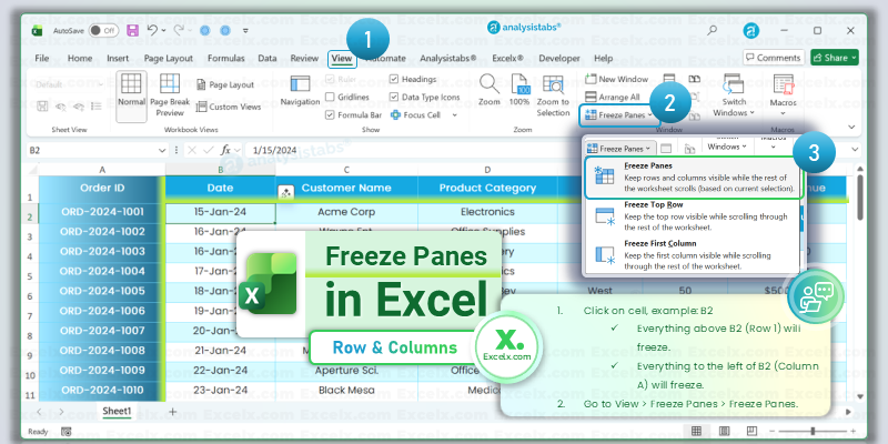
- Click on cell B2 (or whichever cell is just inside your data area).
- Everything above B2 (Row 1) will freeze.
- Everything to the left of B2 (Column A) will freeze.
- Go to View > Freeze Panes > Freeze Panes.
How to Freeze Panes in Excel Mobile (iPhone/Android)
If you are working on a tablet or phone, the interface is different. A common issue users face is not being able to scroll because a pane is locked. Here is “to scroll turn off freeze panes in excel mobile”:
On iPad/Tablet:
1. Go to the View tab.
2. Tap Freeze Panes.
3. Select the option you need (or uncheck it to unfreeze).
On iPhone/Android Phone:
1. Tap the Ribbon icon (or the arrow at the bottom right) to expand the menu.
2. Tap Home to switch tabs and select View.
3. Scroll down to find Freeze Panes.
4. If panes are already frozen and you can’t scroll properly, tap Freeze Panes again to turn it off.
Clarification: “Freezing Formula” vs. “Freezing Panes”
Are you looking for a shortcut to freeze formula in Excel? This is a common mix-up in search results!
- Freeze Panes: Locks the view (Rows/Columns) so they don’t move when you scroll.
- Freeze Formula: Locks a cell reference (e.g., changing ‘A1’ to ‘$A$1’) so it doesn’t change when you drag it.
If you need to lock a formula: Highlight the reference in your formula bar and press the F4 key.
(Read our full guide on Absolute References here).
Excel Freeze Panes Shortcuts
Speed up your workflow with these keyboard shortcuts. Note: For custom selection, ensure you click the correct cell first.
| Action | Shortcut (Windows) |
|---|---|
| Freeze Top Row | Alt + W + F + R |
| Freeze First Column | Alt + W + F + C |
| Freeze Custom / Selected | Alt + W + F + F |
| Unfreeze Panes | Alt + W + F + F (Toggle) |
How to Unfreeze Rows and Columns in Excel
If you made a mistake or want to “fix panes” differently:
- Go to the View tab.
- Click Freeze Panes.
- Select Unfreeze Panes.
Note: This option only appears if panes are currently frozen.
Troubleshooting: Why is Freeze Panes Greyed Out?
If you cannot click the button (it looks disabled or “greyed out”), you are likely in Page Layout View or Cell Editing Mode.
The Fix:
1. Press Esc to ensure you aren’t editing a cell.
2. Go to View > Workbook Views > Click Normal.
Frequently Asked Questions (FAQs)
Q: Can I freeze rows in the middle of the spreadsheet?
A: No. Excel always freezes from the top-down or left-to-right. You cannot freeze “Rows 10-15” while leaving Rows 1-9 scrollable.
Q: How do I make Excel freeze panes print on every page?
A: This is a very common question! Freezing panes only affects the *screen*. To print headers:
1. Go to the Page Layout tab.
2. Click Print Titles.
3. Under “Rows to repeat at top,” select your header row.
Q: Why can’t I scroll past a certain point?
A: You likely froze a large portion of your screen by accident. Go to View > Unfreeze Panes to reset your view.
Q: Why does the line locking my rows look so thick?
A: You likely clicked “Split” instead of “Freeze Panes.” Go to the View tab and click Split to turn it off.
Summary
Whether you need to lock a simple header, freeze selected columns, or fix panes horizontally and vertically, the rule is always the same: **Select the cell below and to the right** of what you want to lock.
Next Step: Now that your view is organized, make sure your data doesn’t break when you move it. Check out our guide on How to Lock Formulas with Absolute References ($).
