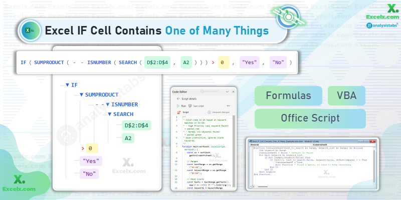
Quick Answer: To check if a cell (e.g., A2) contains any text from a list (e.g., D2:D4), don’t use nested IFs.
Universal Formula (All Excel Versions)
=IF(SUMPRODUCT(--ISNUMBER(SEARCH(D$2:D$4, A2)))>0, "Yes", "No")Modern Excel (Microsoft 365, 2021+)
=IF(OR(ISNUMBER(SEARCH(D$2:D$4, A2))), "Yes", "No")Summary
This guide teaches you how to efficiently check if a cell contains one of many things, helping you move beyond complex and fragile nested IF statements.
We cover every angle on this problem, providing solutions for all types of users and requirements. This includes:
- Universal Formulas: Using
SUMPRODUCTfor maximum compatibility with all Excel versions. - Modern Dynamic Array Formulas: A simpler, more intuitive approach for Microsoft 365.
- Automation Methods: Reusable VBA functions for desktop and Office Scripts for web-based automation.
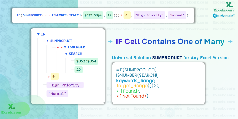
The most reliable formula for universal use, which we’ll break down first, is:
=IF(SUMPRODUCT(--ISNUMBER(SEARCH(D2:D4, A2)))>0, "High Priority", "Normal")Read on to understand each technique and choose the best one for your requirement. 🚀
The Old Way: Why Nested IFs Fail
Let’s say you’re a sales analyst, and you need to categorize incoming customer feedback. Your list of keywords is “poor,” “broken,” and “slow.” The old-school approach would be a monstrous nested IF formula like this:
=IF(ISNUMBER(SEARCH("poor", A2)), "Complaint", IF(ISNUMBER(SEARCH("broken", A2)), "Complaint", IF(ISNUMBER(SEARCH("slow", A2)), "Complaint", "Other")))This is hard to read, a nightmare to update, and breaks easily. If you have ten keywords, this formula becomes a disaster. There’s a much, much better way.
The Goal: One Formula to Check a List
Our goal is to create a single, scalable formula that checks if a cell contains any text from a predefined list. We want a simple “Yes” or “No” (or TRUE/FALSE) that we can easily use in other functions like IF, FILTER, or XLOOKUP.
For this tutorial, we’ll use this sample data: We have a list of transaction descriptions in column A and a list of keywords in column D that we want to flag as “High Priority”.
| A | B | C | D | |
|---|---|---|---|---|
| 1 | Transaction | Priority? | Keywords | |
| 2 | Invoice #482 urgent payment | urgent | ||
| 3 | Shipment delayed: part 9B | overdue | ||
| 4 | Weekly sales summary | critical | ||
| 5 | CRITICAL system failure alert | |||
| 6 | Past due invoice #113 |
The Logic: Combining SEARCH and ISNUMBER
The magic behind this technique lies in two helper functions: SEARCH and ISNUMBER.
SEARCH: This function looks for a substring inside another text string. For example,SEARCH("apple", "An apple a day")returns4. Crucially, if it doesn’t find the text, it returns a#VALUE!error. It’s also case-insensitive.ISNUMBER: This function checks if a value is a number. It conveniently converts any error (like#VALUE!) intoFALSE.
When we use SEARCH with a list of keywords against a single cell, it returns an array of results. For cell A2 (“Invoice #482 urgent payment”) and our keywords in D2:D4:
SEARCH(D2:D4, A2) would evaluate to: {#VALUE!; 15; #VALUE!}
Because “urgent” was found at character 15, but “overdue” and “critical” were not. ISNUMBER turns this into a clean Boolean array:
ISNUMBER({#VALUE!; 15; #VALUE!}) → {FALSE; TRUE; FALSE}
This array is the key. Now we just need to check if it contains at least one TRUE.
Universal Solution: SUMPRODUCT for Any Excel Version
SUMPRODUCT is one of Excel’s most versatile functions. While it’s designed to multiply and sum arrays, we can use it here to count the TRUE values in our Boolean array. It works flawlessly in all versions of Excel.
The Full Formula Breakdown
Here’s the formula to enter in cell B2:
=IF(SUMPRODUCT(--ISNUMBER(SEARCH($D$2:$D$4, A2)))>0, "High Priority", "Normal")Let’s break it down from the inside out:
SEARCH($D$2:$D$4, A2): As we saw, this attempts to find each keyword in cell A2, returning an array of numbers and errors (e.g.,{#VALUE!; 15; #VALUE!}).ISNUMBER(...): Converts that array intoTRUEs andFALSEs (e.g.,{FALSE; TRUE; FALSE}).--: This is the double unary operator. It’s a clever trick that coercesTRUEvalues into1s andFALSEvalues into0s. So{FALSE; TRUE; FALSE}becomes{0; 1; 0}.SUMPRODUCT(...): Sums the items in the numeric array.0 + 1 + 0 = 1.>0: We check if the sum is greater than zero. If it is, at least one keyword was found.1 > 0isTRUE.IF(...): TheIFfunction then returns “High Priority” because the logical test wasTRUE.
How It Works: A Visual Breakdown
Here’s the formula in action. Notice how we use absolute references ($D$2:$D$4) for the keyword list so it stays locked when we drag the formula down.
Modern Excel: Dynamic Arrays Simplify Everything
If you’re using Microsoft 365, Excel 2021, or Excel for the Web, you can leverage the power of dynamic arrays to create a much simpler and more intuitive formula.
The Effortless OR + SEARCH Combo
In modern Excel, functions can handle arrays natively. This means we can use the OR function directly on our ISNUMBER/SEARCH result.
=IF(OR(ISNUMBER(SEARCH($D$2:$D$4, A2))), "High Priority", "Normal")Here, OR({FALSE; TRUE; FALSE}) directly evaluates to TRUE, no SUMPRODUCT or double unary needed! It’s cleaner and easier for others to understand.
Processing a Full Column with BYROW
Want to get even fancier? The BYROW function lets you process an entire range of data with a single formula in a single cell.
=BYROW(A2:A6, LAMBDA(row, IF(OR(ISNUMBER(SEARCH(D2:D4, row))), "High Priority", "Normal")))You enter this formula only in cell B2, and it automatically spills the results down for the entire range A2:A6. This is incredibly efficient for large datasets and dashboards.
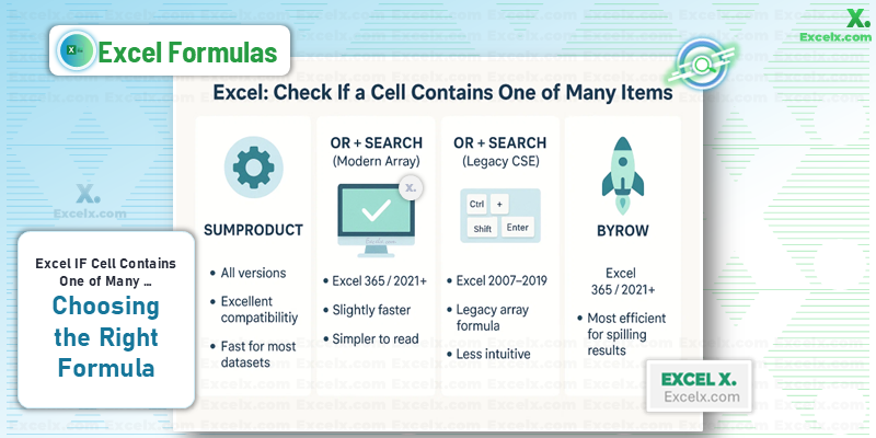
Performance & Version Notes
For most spreadsheets, any of these methods are lightning-fast. However, on tens of thousands of rows, there are minor differences.
| Method | Excel Version | Performance Note |
|---|---|---|
| SUMPRODUCT | All Versions | Excellent compatibility. Very fast on most datasets. |
| OR (with Ctrl+Shift+Enter) | Excel 2007-2019 | This is an older array formula style. It works but is less intuitive. |
| OR (Dynamic Array) | Microsoft 365, 2021+ | Slightly faster than SUMPRODUCT on very large datasets. The preferred modern method. |
| BYROW | Microsoft 365, 2021+ | The most efficient for spilling results down an entire column with one formula. |
Automation Corner: VBA and Office Scripts
Custom VBA Function for Reusability
If you do this check often, a custom VBA function (UDF) can be a lifesaver. Press ALT + F11, insert a new module, and paste this code. The below VBA UDF that returns TRUE if a Cell’s text contains any keyword from a range (case-insensitive); FALSE otherwise. Blank keywords are ignored.
Function ContainsOneOf(text_to_search As Range, keyword_list As Range) As Boolean
    Dim keyword As Range
    ContainsOneOf = False ' Default to False
    For Each keyword In keyword_list
        If Not IsEmpty(keyword.Value) Then
            If InStr(1, text_to_search.Value, keyword.Value, vbTextCompare) > 0 Then
                ContainsOneOf = True
                Exit Function ' Found a match, no need to keep searching
            End If
        End If
    Next keyword
End Function
Now you can use it in your worksheet like any other function:
=IF(ContainsOneOf(A2, $D$2:$D$4), "Yes", "No")Office Scripts for Web-Based Automation
For Excel on the Web, you can use Office Scripts (TypeScript) for a modern automation solution. This can be run on a schedule or triggered by a button.
Keyword Priority Labeler
Checks A2:A6 against keywords in D2:D4 (case-insensitive) and writes High Priority or Normal to H2:H with a header in H1; ignores blank keywords and logs completion.
/**
 * Script Objective
 * - Label each transaction in A2:A6 as "High Priority" if it contains any keyword from D2:D4 (case-insensitive); otherwise "Normal".
 * - Write header to H1 and results to H2:H.
 * - Ignore blank keywords; substring matching.
 * - Non-destructive: reads A/D, writes H (and status note in J1), logs success.
 */

function main(workbook: ExcelScript.Workbook) {
    // Active worksheet
    const selectedSheet = workbook.getActiveWorksheet();

    // Input ranges:
    // A2:A6 → texts to check
    // D2:D4 → keyword list (partial-match substrings)
    const textRange = selectedSheet.getRange("A2:A6");
    const keywordRange = selectedSheet.getRange("D2:D4");

    // Read values from A2:A6 → flatten to string array
    const texts = textRange.getTexts().map(r => (r[0] ?? "").toString());

    // Read values from D2:D4 → trim → drop blanks
    const keywords = keywordRange
        .getTexts()
        .map(r => (r[0] ?? "").toString().trim())
        .filter(s => s.length > 0);

    // Case-insensitive matching: pre-lowercase all keywords
    const lowerKeywords = keywords.map(k => k.toLowerCase());

    // For each text in A2:A6, check if any keyword occurs as a substring
    // Return a 2D array suitable for setValues: [["High Priority"], ["Normal"], ...]
    const results = texts.map(t => {
        const hay = t.toLowerCase(); // case-insensitive haystack
        const match = lowerKeywords.some(k => hay.indexOf(k) !== -1); // true if any keyword found
        return [match ? "High Priority" : "Normal"];
    });

    // Write header in H1
    selectedSheet.getRange("H1").setValue("Priority? (Script)");

    // Write results starting at H2 (downward).
    // getResizedRange(rowsDelta, colsDelta): rowsDelta = results.length - 1 to cover all rows
    if (results.length > 0) {
        selectedSheet.getRange("H2").getResizedRange(results.length - 1, 0).setValues(results);
    }

    // Optional status stamp in J1 and console
    selectedSheet.getRange("J1").setValue("Excelx.com: script ran successfully");
    console.log("Excelx.com script ran successfully");
}
Keyword Priority Highlighter
Color-code transactions by priority. This Office Script checks each text in A2:A6 against keywords in D2:D4 (case-insensitive) and fills the A-cells pastel red when a match is found (High Priority) or pastel green when not (Normal). Blank keywords are ignored; only cell fills are changed.
/**
 * Color-code A2:A6 based on keyword matches in D2:D4:
 * - High Priority (any keyword found) → pastel red
 * - Normal (no keywords found)        → pastel green
 * Case-insensitive; ignores blank keywords.
 */

function main(workbook: ExcelScript.Workbook) {
    const ws = workbook.getActiveWorksheet();

    // Ranges
    const textRange = ws.getRange("A2:A6");
    const keywordRange = ws.getRange("D2:D4");

    // Read inputs
    const texts = textRange.getTexts().map(r => (r[0] ?? "").toString());
    const keywords = keywordRange
        .getTexts()
        .map(r => (r[0] ?? "").toString().trim())
        .filter(s => s.length > 0);
    const lowerKeywords = keywords.map(k => k.toLowerCase());

    // Colors
    const PASTEL_RED = "#FEE2E2";   // High Priority
    const PASTEL_GREEN = "#D1FAE5"; // Normal

    // Apply fills row-by-row
    const rows = textRange.getRowCount();
    for (let i = 0; i < rows; i++) { const cell = textRange.getCell(i, 0); const hay = texts[i].toLowerCase(); const match = lowerKeywords.some(k => hay.indexOf(k) !== -1);

        const fill = cell.getFormat().getFill();
        fill.clear(); // reset existing fill
        fill.setColor(match ? PASTEL_RED : PASTEL_GREEN);
    }

    ws.getRange("J1").setValue("Excelx.com: colors updated");
    console.log("Excelx.com: colors updated");
}
Common Pitfalls and Smart Fixes
- Problem: You get a
#VALUE!error.- Reason: You forgot to wrap
SEARCHinsideISNUMBER. TheSEARCHfunction returns an error if a keyword isn’t found, and this error will break your whole formula unlessISNUMBERcatches it.
- Reason: You forgot to wrap
- Problem: The formula isn’t finding text that you can clearly see (e.g., “apple” vs “Apple”).
- Reason: You need a case-sensitive search. You used
SEARCH(case-insensitive) instead ofFIND(case-sensitive). - Fix: Simply replace
SEARCHwithFINDin any of the formulas above....SUMPRODUCT(--ISNUMBER(FIND(...
- Reason: You need a case-sensitive search. You used
- Problem: Your keyword list has blank cells causing weird results.
- Fix: While the VBA example handles this, a formula-based fix is to
FILTERyour keyword list first in a helper column or directly in the formula if you have Microsoft 365:...SEARCH(FILTER(D:D, D:D<>""), A2)...
- Fix: While the VBA example handles this, a formula-based fix is to
Advanced Scenarios & Variations
Case-Sensitive Matches with FIND
As mentioned, if you need to distinguish between “ID” and “id”, simply swap SEARCH for FIND.
Universal FIND Formula:
=IF(SUMPRODUCT(--ISNUMBER(FIND($D$2:$D$4, A2)))>0, "Yes", "No")Accessibility: Using Named Ranges
Formulas can get hard to read. Using Named Ranges makes them dramatically clearer.
- Select your keyword list (e.g.,
D2:D4). - Go to the Formulas tab > Define Name.
- Name it something intuitive, like
KeywordList.
Now your formula becomes self-documenting:
=IF(OR(ISNUMBER(SEARCH(KeywordList, A2))), "High Priority", "Normal")This is much easier for you and your colleagues to understand a year from now!
Next Steps in Your Learning Path
Mastering this technique opens up a world of possibilities. Here’s where to go next:
- Count Instead of Flagging: Adapt the
SUMPRODUCTpart to count how many rows contain a keyword:=SUMPRODUCT(--(ISNUMBER(SEARCH(KeywordList, A2:A100))>0)) - Extract the Keyword: Use
XLOOKUPorFILTERwith this logic to not just flag a row, but return which keyword was found. - Combine with Other Criteria: Add more conditions to your
SUMPRODUCTorFILTERfunctions to create powerful, multi-condition summaries.
FAQs
How do I check if a cell contains text from a list in Excel?
The best way is to combine ISNUMBER and SEARCH to look for multiple items. Use this formula, where A1 is the cell to check and list is the range containing your text values: =IF(SUMPRODUCT(--ISNUMBER(SEARCH(list, A1)))>0, "Found", "Not Found").
How do you write an IF OR statement with text in Excel?
For checking if a cell contains one of many substrings (partial text), you can’t use IF(OR(A1="text1", A1="text2"...)) as that only works for exact matches. For partial matches in modern Excel, use =IF(OR(ISNUMBER(SEARCH(list, A1))), "Yes", "No"). For older versions, the SUMPRODUCT method is the standard.
Can an IF statement search for partial text in Excel?
Yes, but not by itself. You need to combine IF with SEARCH (or FIND) and ISNUMBER. A simple formula is =IF(ISNUMBER(SEARCH("partial_text", A1)), "Yes", "No"). This article expands that logic to search for a whole list of partial text strings.
Download the Examples File – Practice Workbook
To see all these formulas in action and try them yourself, download the companion Excel file. It includes the sample data, all the formulas, and the VBA custom function.
