Top 10 Excel Errors and How to Fix Them: Ultimate Excel Troubleshooting Guide

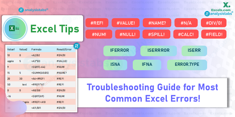
Struggling with cryptic Excel error codes like #REF!, #VALUE!, #NAME?, #N/A, #DIV/0!, #NUM!, #NULL!, #SPILL!, #CALC!, and #FIELD!? You’re not alone. In this ultimate Excel troubleshooting guide, we demystify these common errors with clear, step-by-step fixes, expert tips, and advanced troubleshooting techniques. Whether you’re dealing with broken references or unexpected calculations, this comprehensive post will equip you with the knowledge to transform frustrating errors into seamless, reliable spreadsheets.

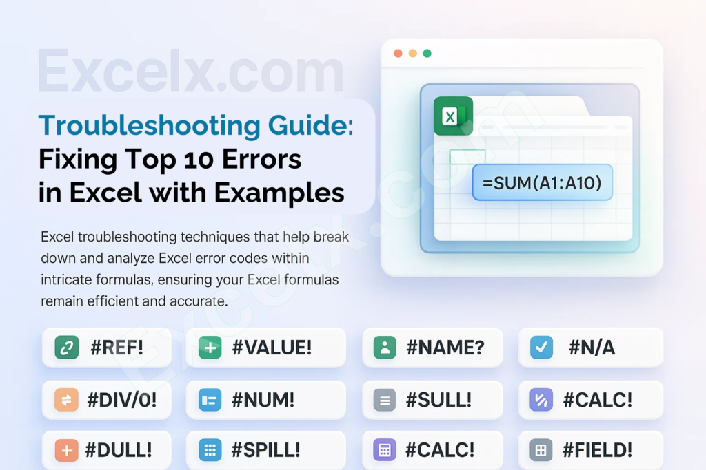
Excel error codes can be confusing, frustrating, and time-consuming, but mastering them is essential for anyone who works with spreadsheets. In this ultimate guide, you’ll learn how to fix the top 10 Excel errors: from #REF! to #FIELD! including: step-by-step instructions for auditing complex formulas, and advanced troubleshooting techniques to build error-free, reliable workbooks.

1. #REF! Error

No matter how meticulously you build your spreadsheet, you might encounter #REF! when Excel can’t find a valid cell reference. This error typically crops up if you delete rows or columns that a formula depends on, or if you copy/paste formulas in a way that breaks references. Understanding how to fix #REF! is crucial for anyone who frequently edits and rearranges complex worksheets.

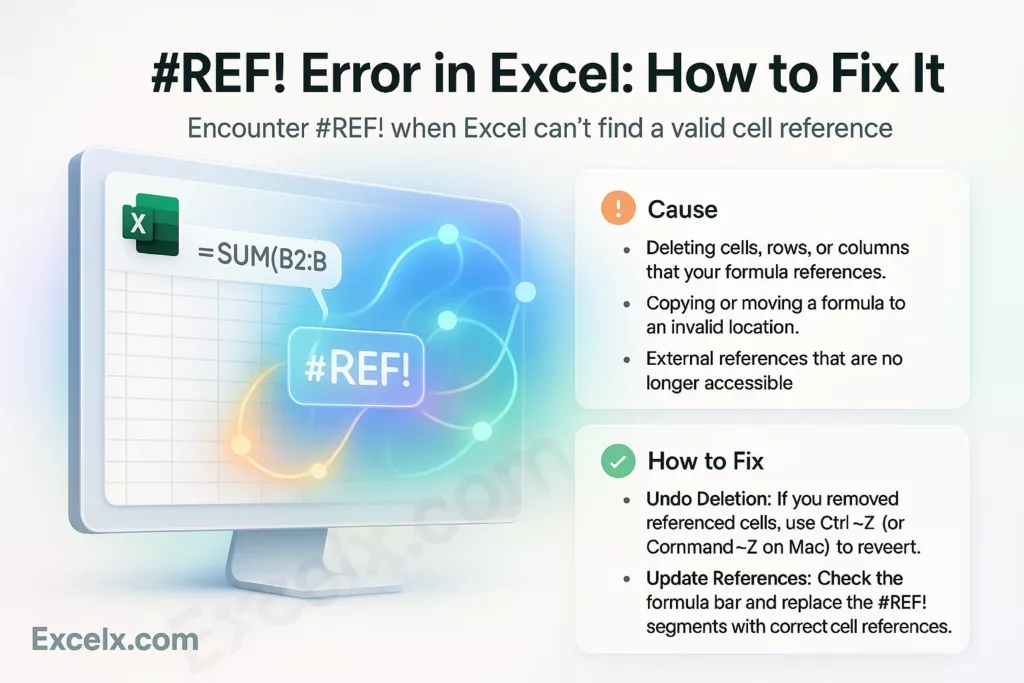
Cause

• Deleting cells, rows, or columns that your formula references.
• Copying or moving a formula to an invalid location.
• External references that are no longer accessible.

How to Fix

1. Undo Deletion: If you removed referenced cells, use Ctrl + Z (or Command + Z on Mac) to revert.
2. Update References: Check the formula bar and replace the #REF! segments with the correct cell references.
3. Use Named Ranges: This practice prevents references from breaking when you delete or move cells.

2. #VALUE! Error

#VALUE! is Excel’s way of saying “I expected a certain data type, but got something else.” Often it appears if your formula tries to perform arithmetic on text or if you inadvertently include a range with mixed content. It’s also a common sight when using functions that require numbers but find dates, text strings, or blank cells instead.

Cause

• Applying arithmetic operators to text cells or non-numeric data.
• Passing the wrong argument type to a function (e.g., using a string instead of a number).
• Inconsistent data formats in the range.

How to Fix

1. Check Data Types: Convert text to numbers (use VALUE() or the “Text to Columns” feature).
2. Trim Text: Use TRIM() to remove hidden spaces that might be interpreted as text.
3. Validate Arguments: Ensure each function argument is of the correct type (number, text, etc.).

3. #NAME? Error

Encountering #NAME? typically means Excel doesn’t recognize something in your formula—maybe a misspelled function name, an undefined named range, or forgotten quotation marks around text. If your formula looks perfect yet you still see #NAME?, double-check each function’s spelling and confirm any named ranges actually exist in your workbook. This error crops up frequently, but is usually one of the quickest to fix once you know where to look.

Cause

• Typo in a function name (e.g., =SUMM(A1:A5) instead of =SUM(A1:A5)).
• Named range doesn’t exist or is spelled incorrectly.
• Unquoted text (Excel interprets it as an undefined name).

How to Fix

1. Check Spelling: Compare your function names to Excel’s Function Library.
2. Manage Named Ranges: Go to Formulas > Name Manager and verify they’re correct.
3. Enclose Text in Quotes: For text literals, wrap them in quotes (e.g., “Hello”).

4. #N/A Error

If your lookup formulas—like VLOOKUP, HLOOKUP, INDEX MATCH, or XLOOKUP—come up empty, you’ll likely see #N/A. This indicates “not available,” meaning Excel couldn’t find a match for your lookup value. While it can be frustrating, this error is often a helpful clue that your data might be missing, mismatched, or suffering from hidden inconsistencies (like trailing spaces or inconsistent data formats).

Cause

• Lookup functions fail to find a matching value.
• Typos or trailing spaces in your lookup value vs. your data list.
• Data not in the expected sort order when using approximate matching.

How to Fix

1. Check the Spelling: Ensure your lookup value and the data source match exactly.
2. Use IFERROR or IFNA: Wrap your lookup in =IFERROR(…) to display a custom message instead of #N/A.
3. Switch to Exact Match: Use FALSE (or 0) in VLOOKUP/HLOOKUP if approximate match is not intended.

5. #DIV/0! Error

#DIV/0! is Excel’s version of “You can’t divide by zero.” It can show up if a formula attempts to divide by a blank cell, or a cell containing zero. While straightforward, this error can suddenly appear in dashboards or summary sheets when data changes. Knowing how to handle it gracefully is essential for maintaining professional-looking outputs.

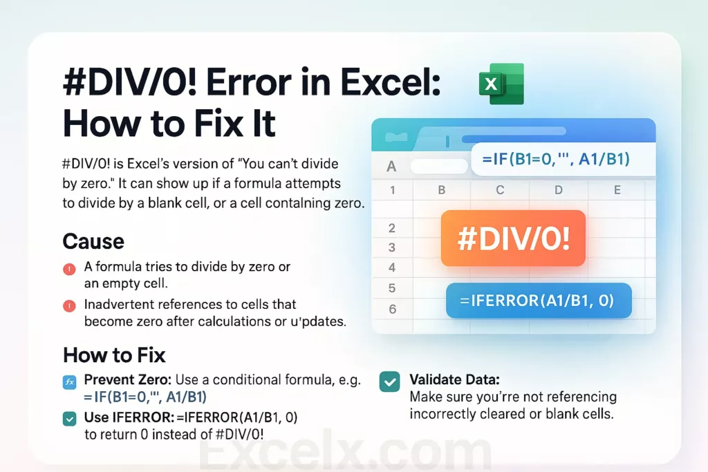
Cause

• A formula tries to divide by zero or an empty cell.
• Inadvertent references to cells that become zero after calculations or updates.

How to Fix

1. Prevent Zero: Use a conditional formula, e.g. =IF(B1=0,””, A1/B1).
2. Use IFERROR: =IFERROR(A1/B1, 0) to return 0 instead of #DIV/0!.
3. Validate Data: Make sure you’re not referencing incorrectly cleared or blank cells.

6. #NUM! Error

Whenever Excel struggles with an invalid numeric value—like a number that’s too large for it to handle, a negative number where a positive is expected, or an impossible calculation—it raises #NUM!. It can happen with certain functions (like SQRT for negative values) or if you enter an extremely large exponent. While it’s less common than #REF! or #VALUE!, it’s just as crucial to understand for advanced numerical tasks.

Cause

• Functions like SQRT or LOG used on negative values.
• Excessively large numbers or out-of-range calculations.
• Improper arguments in financial functions (like IRR or RATE).

How to Fix

1. Check Function Requirements: Make sure you’re not passing negative values to functions that require non-negative inputs.
2. Reduce Data Range: If you have extremely large numbers, confirm they’re valid or break them down.
3. Validate Financial Inputs: For IRR, RATE, or NPER, ensure your parameters make mathematical sense.

7. #NULL! Error

Although not as frequently encountered, #NULL! can pop up if you accidentally use a space where Excel expects a comma or colon, especially when referencing multiple ranges. In Excel, a space in a formula often signifies an “intersection” operator (meaning overlapping cells). If no intersection exists between the specified ranges, you get #NULL!. Understanding how referencing syntax works is the key to avoiding this lesser-known error.

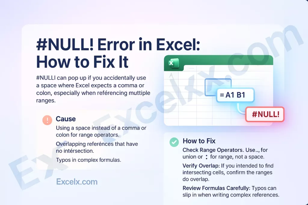
Cause

• Using a space instead of a comma or colon for range operators.
• Overlapping references that have no intersection.
• Typos in complex formulas.

How to Fix

1. Check Range Operators: Use , for union or : for range, not a space.
2. Verify Overlap: If you intended to find intersecting cells, confirm the ranges do overlap.
3. Review Formulas Carefully: Typos can slip in when writing complex references.

8. #SPILL! Error

If you’re using the newer dynamic array functions in Excel (Microsoft 365 or Excel 2021+), you might see #SPILL! Error when Excel can’t place the full result of a formula into the worksheet. This happens when other data or formatting blocks the cells that the dynamic array wants to “spill” into. Knowing how to unblock or relocate that data ensures you fully harness the power of dynamic arrays.

Cause

• A dynamic array formula returns multiple values, but adjacent cells are occupied.
• Merged cells or formatting blocks the spill range.
• The formula’s output is larger than the available free space.

How to Fix

1. Clear or Move Conflicting Cells: Check the cells the array would fill; remove or relocate data.
2. Choose a Different Location: Place the formula somewhere with enough space to “spill.”
3. Watch Merged Cells: Unmerge or adjust them so they don’t block dynamic arrays.

9. #CALC! Error

#CALC! is relatively new, often associated with dynamic array operations. It signifies a calculation error that can’t be classified under more common codes like #VALUE! or #REF!. For instance, if you use an invalid argument in a dynamic array function or try to combine them in ways Excel doesn’t allow, #CALC! might appear. Troubleshooting this often means double-checking function compatibility and formula logic.

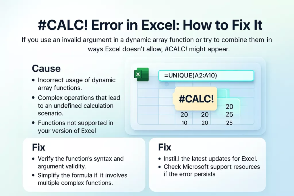
Cause

• Incorrect usage of dynamic array functions.
• Complex operations that lead to an undefined calculation scenario.
• Functions not supported in your version of Excel.

How to Fix

1. Review Dynamic Array Functions: Make sure your formula is supported and you’re using correct arguments.
2. Upgrade Excel: If you’re on an older version, certain array operations might not work.
3. Simplify: If the formula is extremely complex, try breaking it into smaller pieces to locate the error.

10. #FIELD! Error

#FIELD! is another newer error that appears in Excel when you reference a field that doesn’t exist—often within linked data types (like Stocks and Geography) or if you’re pulling data from external sources. If you’re working with data types or Power Query–style transformations, you might encounter it. Solving #FIELD! typically involves double-checking your field names, spelling, or the structure of the external data you’re referencing.

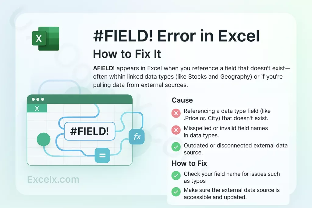
Cause

• Referencing a data type field (like .Price or .City) that doesn’t exist.
• Misspelled or invalid field names in data types.
• Outdated or disconnected external data source.

How to Fix

1. Verify Field Names: Ensure you’ve spelled field attributes correctly (e.g., .Price, .Population, etc.).
2. Refresh Data: If you’re using external data types, refresh the connection to ensure the fields are still valid.
3. Use Data Types Pane: In Excel 365, check the “Data Types” tab to see available fields.

Understanding Excel’s Error Handling Mechanisms

Excel’s built-in logic is designed to catch Excel errors before they disrupt your workflow. In this section, we explore how Excel evaluates formulas, detects issues like #REF! and #VALUE!, and helps you fix Excel errors. Mastering these mechanisms is essential for effective Excel troubleshooting and robust Excel formulas.

• Provides the foundation for understanding common Excel errors.
• Explains the importance of knowing how Excel processes formulas.
• Helps users learn how to fix Excel errors efficiently.

How Excel Processes Errors

• Formula Evaluation: Excel examines every cell reference, operator, and function.
• Error Detection: If a component is invalid, Excel interrupts the calculation and displays an error code.
• Troubleshooting: Use built-in tools to trace and correct errors.

Using Error Functions

• IFERROR, IFNA, and ISERROR are key functions for capturing errors.
• They allow you to display custom messages and alternative values.
• Tip: Implement these functions in your formulas to prevent disruptions from common Excel error codes.

Excel Error Handling Functions

Excel error handling functions are essential for robust Excel troubleshooting. They allow you to catch, evaluate, and manage Excel errors effectively, ensuring that your formulas remain accurate and user-friendly. In this section, we cover key functions such as IFERROR, ISERROR, IFNA, ISNA, ISERR, and ERROR.TYPE, complete with syntax, examples, and use cases.

IFERROR Function

• Purpose: Catches errors in a formula and returns a custom result instead of the error code.
• Syntax: =IFERROR(value, value_if_error)
• Example:
  • Formula: =IFERROR(A2/B2, “Error in division”)
  • Explanation: If A2/B2 produces an error (e.g., #DIV/0!), the formula returns “Error in division”.
• Use Case: Ideal for simplifying formulas by preventing error codes from disrupting your workflow.

ISERROR Function

• Purpose: Checks whether a value results in any error, returning TRUE if an error is present and FALSE otherwise.
• Syntax: =ISERROR(value)
• Example:
  • Formula: =ISERROR(A2/B2)
  • Explanation: Returns TRUE if A2/B2 causes an error like #DIV/0!, #VALUE!, etc.
• Use Case: Useful for conditionally handling errors within larger formulas.

IFNA Function

• Purpose: Specifically traps the #N/A error and returns an alternative value.
• Syntax: =IFNA(value, value_if_na)
• Example:
  • Formula: =IFNA(VLOOKUP(C2, A2:B10, 2, FALSE), “Not Found”)
  • Explanation: If the lookup fails (returning #N/A), the formula outputs “Not Found”.
• Use Case: Particularly beneficial in lookup scenarios to provide a user-friendly message when no match is found.

ISNA Function

• Purpose: Tests explicitly for the #N/A error.
• Syntax: =ISNA(value)
• Example:
  • Formula: =ISNA(VLOOKUP(“abc”, A2:B10, 2, FALSE))
  • Explanation: Returns TRUE if the lookup results in #N/A, otherwise FALSE.
• Use Case: Ideal for distinguishing #N/A errors from other error types.

ISERR Function

• Purpose: Checks for any error except #N/A.
• Syntax: =ISERR(value)
• Example:
  • Formula: =ISERR(A2/B2)
  • Explanation: Returns TRUE if A2/B2 results in an error other than #N/A.
• Use Case: Use this function when you want to handle all error types except #N/A, which might be handled separately with ISNA or IFNA.

ERROR.TYPE Function

• Purpose: Returns a numeric value corresponding to the type of error present in a cell.
• Syntax: =ERROR.TYPE(error_value)
• Example:
  • Formula: =ERROR.TYPE(A2/B2)
  • Explanation: If A2/B2 results in #DIV/0!, the function might return a specific number (e.g., 2 for #DIV/0!). Refer to Excel’s documentation for the complete list of error type numbers.
• Use Case: Useful for diagnosing errors programmatically by identifying their type via a numeric code.

Additional Tips for Error Handling

• Combine with Data Validation: Enhance error resilience by pairing error functions with strict data validation rules.
• Nested Functions: Consider nesting error functions for complex scenarios to manage multiple potential error types.
• Test Thoroughly: Validate your error handling across varied data inputs to ensure robust performance and reliability.

These error handling functions are powerful tools in your Excel toolkit. They allow you to create formulas that are not only error-resistant but also user-friendly and professional in appearance.

 

Excel’s Built-In Error Checking and Auditing Tools

Excel’s integrated tools streamline the process of identifying and fixing Excel errors. This section covers how to use features like Error Checking, Trace Precedents, and Evaluate Formula for effective Excel troubleshooting and accurate Excel formulas. These tools are essential for diagnosing and resolving Excel error codes.

Error Checking Features

• Automatic Scanning: Excel automatically flags potential issues.
• Tooltip Explanations: Brief descriptions help you understand each error.
• Quick Fix Suggestions: Provides immediate solutions for common Excel errors.

Formula Auditing Tools

• Trace Precedents/Dependents: Visualize the relationships between cells.
• Evaluate Formula: Step through your formula to locate errors.

List of Tools:

1. Trace Precedents
2. Trace Dependents
3. Evaluate Formula

Practical Usage

• Access Tools: Navigate to the Formulas tab.
• Implement Auditing: Use the auditing tools for a systematic review.
• Resolve Issues: Follow the suggestions to fix Excel errors

Preventative Measures: Best Practices for Error-Free Spreadsheets

Preventative strategies are key to avoiding Excel errors and ensuring smooth performance. This section outlines best practices—such as data validation, organized design, and documentation—to help you fix Excel errors before they occur, leading to efficient Excel troubleshooting and flawless Excel formulas.

Designing with Clarity

• Organize Data: Use clearly labelled tables and consistent formatting.
• Document Formulas: Write clear notes and comments in your workbook.

Benefits:

1. Enhanced readability
2. Fewer errors
3. Easier maintenance

Implementing Data Validation

• Set Validation Rules: Restrict cell inputs to expected data types.
• Create Drop-Down Menus: Use lists to ensure consistency.
• Key Points: Reduces Excel errors like #VALUE! and #N/A.

Step-by-Step Guide to Auditing Complex Formulas

Auditing complex formulas is a systematic way to locate and fix Excel errors. This section provides a step-by-step guide using Excel troubleshooting techniques that help break down and analyze Excel error codes within intricate formulas, ensuring your Excel formulas remain efficient and accurate.

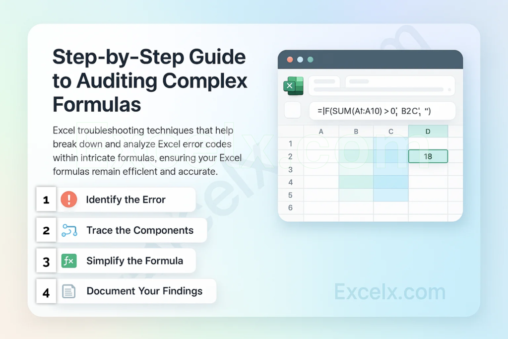
Step 1: Identify the Error

• Recognize Error Codes: Determine if it’s #REF!, #DIV/0!, etc.
• List of Common Errors: #REF!, #VALUE!, #DIV/0!

Step 2: Trace the Components

• Use Auditing Tools: Apply Trace Precedents and Dependents.
• Break Down the Formula: Isolate parts to pinpoint the error source.
• Document Observations: Record the sequence of steps and findings.

Step 3: Simplify the Formula

• Divide Complex Calculations: Break into intermediate steps.
• Rebuild for Clarity: Combine simpler formulas to maintain readability.
• Advantages: Easier error detection and Excel troubleshooting.

Step 4: Document Your Findings

• Maintain a Log: Track errors and solutions.
• Use Comments: Insert notes directly in the workbook.
• Benefits: Future reference, Improved team collaboration

Leveraging Named Ranges and Structured References

Utilizing named ranges and structured references simplifies your work and helps fix Excel errors. This section explains how these features improve Excel formulas by ensuring consistency and preventing common error codes like #REF!. Adopting these techniques is crucial for efficient Excel troubleshooting.

Benefits of Named Ranges

• Clarity in Formulas: Replace cell addresses with descriptive names.
• Enhanced Flexibility: Automatically adjust when data shifts.
• List of Benefits: Reduced errors, Improved readability, Easier maintenance

Using Structured References in Tables

• Dynamic Ranges: Structured references update automatically.
• Improved Accuracy: Reduces risk of Excel error codes when rows or columns change.
• Advantages: Consistent formulas, Simplified data management

Advanced Troubleshooting Techniques for Dynamic Array Formulas

Dynamic arrays introduce new challenges like #SPILL! and #CALC! errors. This section offers advanced troubleshooting techniques to fix Excel errors in dynamic array formulas, ensuring your Excel formulas run smoothly. Learn how to resolve these issues using modern Excel troubleshooting strategies.

Resolving #SPILL! Errors

• • Clear Blockages: Remove any obstructing data from the spill range.
  • Check for Merged Cells: Unmerge cells that hinder dynamic arrays.

Steps to Resolve:

1. Identify the spill range
2. Clear conflicts
3. Reapply the formula

Addressing #CALC! Errors

1. Review Formula Logic: Check for incompatible operations.
2. Update Functions: Ensure all dynamic functions are supported.
3. Troubleshooting Steps: Break down the formula to locate errors.

Best Practices for Dynamic Arrays

1. Plan Your Layout: Ensure adequate space for spilled data.
2. Test Incrementally: Build your formula step by step.
3. Key Takeaways: Reduced error rates, Improved efficiency

Optimizing Data Validation to Minimize Errors

Optimizing data validation is essential for preventing Excel errors and ensuring accurate data entry. In this section, we explain how to use validation rules and drop-down menus to fix Excel errors and streamline Excel troubleshooting while maintaining robust Excel formulas.

Setting Up Validation Rules

1. Define Acceptable Inputs: Limit data types and ranges.
2. Configuration Tips: Use whole number or date restrictions, Apply input messages and error alerts

Using Drop-Down Menus

1. Create Lists: Generate drop-down menus for consistent data entry.
2. Benefits: Minimizes Excel errors like typos and mismatched entries.

Implementation Steps:

1. Select the cell range
2. Apply data validation
3. Define list options

Case Studies: Real-World Examples of Excel Error Resolutions

Real-world examples provide valuable insights into fixing Excel errors effectively. This section features detailed case studies where professionals successfully resolved common Excel error codes. Learn from practical Excel troubleshooting scenarios to enhance your skills in creating robust Excel formulas.

Financial Analysis Error Resolution

Scenario: A financial analyst encountered #NUM! errors.

Steps Taken:

1. Identified erroneous data
2. Corrected inputs
3. Implemented error checks

Outcome:

• • Improved calculation accuracy and data integrity.

Marketing Dashboard Error Fixes

• Scenario: A marketing team resolved #DIV/0! and #N/A errors.
• Approach:

1. Applied conditional formulas
2. Validated lookup data

• Result: Enhanced dashboard reliability and user experience.

Integrating Power Query and Other Advanced Excel Tools for Cleaner Data

Integrating advanced tools like Power Query transforms data management and helps fix Excel errors. This section covers how Power Query, pivot tables, and data models enhance Excel troubleshooting and produce accurate Excel formulas while preventing common error codes.

Using Power Query for Data Cleaning

• Import and Transform: Cleanse data before it reaches your worksheet.
• Benefits:
  • Prevents Excel errors such as #VALUE!.
• Key Steps:

• Import data
• Apply cleansing filters
• Load clean data into Excel

Leveraging Pivot Tables for Error Detection

• Analyze Data: Use pivot tables to spot anomalies and errors.
• Advantages:

• 1. • Summarizes large data sets
     • Identifies inconsistencies quickly

• Implementation:
  • Create pivot tables to cross-check data integrity.

Frequently Asked Questions (FAQs) on Excel Errors

This FAQ section addresses 25 of the most popular questions on Excel errors, offering actionable insights to fix Excel errors and improve Excel troubleshooting. Discover common Excel error codes, learn how to correct faulty Excel formulas, and gain tips for maintaining smooth, error-free spreadsheets with these expert answers.

1. What are Excel errors?
   Answer: Excel errors are codes like #REF!, #VALUE!, #DIV/0!, etc., that indicate issues in formulas, cell references, or data types. They help diagnose problems and guide you to fix Excel errors effectively.
2. What causes the #REF! error in Excel?
   Answer: The #REF! error typically occurs when a formula references a cell that has been deleted or moved, breaking the cell reference and resulting in an invalid formula.
3. What does the #VALUE! error mean?
   Answer: The #VALUE! error indicates that a formula is receiving an argument of the wrong type, such as text instead of a number, preventing proper calculation.
4. How can I fix the #DIV/0! error?
   Answer: The #DIV/0! error occurs when a number is divided by zero. Resolve it by ensuring denominators are non-zero or by using error-handling functions like IFERROR.
5. What does the #NAME? error indicate?
   Answer: The #NAME? error appears when Excel does not recognize text in a formula—often due to typos in function names or missing quotation marks around text strings.
6. How do I resolve the #N/A error in lookup functions?
   Answer: The #N/A error occurs when a lookup function cannot find a matching value. Verify your data for consistency and consider using IFNA to handle missing values gracefully.
7. What causes the #NUM! error?
   Answer: The #NUM! error arises from invalid numeric operations, such as calculating the square root of a negative number or exceeding Excel’s numerical limits.
8. Why do I get a #NULL! error?
   Answer: The #NULL! error appears when an expected intersection of cell ranges does not exist, often due to incorrect use of range operators or syntax errors.
9. How do I fix the #SPILL! error?
   Answer: The #SPILL! error happens when a dynamic array formula’s result is blocked by adjacent data. Clear or reposition the obstructing cells to allow the formula to spill.
10. What does the #CALC! error mean?
    Answer: The #CALC! error indicates a calculation issue, often in dynamic arrays or complex formulas, where Excel cannot complete the computation due to incompatible operations.
11. How can I fix the #FIELD! error?
    Answer: The #FIELD! error occurs when a formula references a non-existent field in linked data. Verify field names and refresh data connections to resolve the error.
12. How does the IFERROR function help manage errors?
    Answer: IFERROR traps errors in formulas and returns an alternative value or message, ensuring your Excel formulas remain clean and user-friendly even when errors occur.
13. What are the most common causes of Excel errors?
    Answer: Common causes include invalid cell references, data type mismatches, syntax errors, issues with dynamic arrays, and problems with external data connections.
14. How can I prevent Excel errors from occurring?
    Answer: Prevent errors by using data validation, organized layouts, named ranges, structured references, and regular formula auditing to catch issues before they affect your calculations.
15. What is data validation in Excel?
    Answer: Data validation restricts cell inputs to specific types or ranges, ensuring that only acceptable values are entered, which reduces the risk of errors in your calculations.
16. How do I use the Trace Precedents tool?
    Answer: The Trace Precedents tool visually displays the cells that contribute to a formula’s result, helping you pinpoint where an error might be originating.
17. What is the purpose of the Evaluate Formula feature?
    Answer: Evaluate Formula allows you to step through each part of a formula, showing intermediate results so you can identify exactly where an error occurs during calculation.
18. What are dynamic arrays in Excel?
    Answer: Dynamic arrays are formulas that return multiple values and spill them into adjacent cells automatically. They require careful layout planning to avoid errors like #SPILL!.
19. How do named ranges assist in troubleshooting?
    Answer: Named ranges replace cell references with descriptive names, making formulas easier to understand and maintain, which minimizes the occurrence of Excel errors.
20. What are structured references and how do they work?
    Answer: Structured references are used in Excel tables to refer to data by column names. They adjust automatically when data is added or removed, helping to prevent reference errors.
21. How do I set up data validation rules?
    Answer: Select a cell range, navigate to the Data tab, choose Data Validation, and define criteria (e.g., specific numbers, dates, or lists) to ensure only acceptable data is entered.
22. How can Power Query reduce Excel errors?
    Answer: Power Query cleans and transforms data before it enters Excel, standardizing formats and removing inconsistencies to prevent errors in Excel formulas and improve data integrity.
23. What best practices help minimize Excel errors?
    Answer: Best practices include clear data organization, using data validation, employing named ranges and structured references, auditing formulas regularly, and documenting your work thoroughly.
24. How do I handle errors in lookup functions?
    Answer: Use functions like IFERROR or IFNA with lookup formulas (e.g., VLOOKUP) to return custom messages or alternative values when no match is found, minimizing the impact of #N/A errors.
25. Where can I find additional resources on Excel error troubleshooting?
    Answer: Additional resources include Microsoft Support, Excel forums, online tutorials, and expert blogs dedicated to Excel troubleshooting, which offer comprehensive guides to fix Excel errors and optimize your Excel formulas.

Conclusion

Mastering Excel error codes—from #REF! and #VALUE! to #FIELD!—is key to efficient spreadsheet management. By understanding the causes and applying proven fixes, you can transform errors into valuable troubleshooting opportunities. Use built-in auditing tools, robust error handling functions like IFERROR, ISERROR, IFNA, ISNA, ISERR, and ERROR.TYPE, and best practices to build resilient, error-free workbooks. Embrace these strategies to boost your Excel skills, streamline your workflow, and ensure your data remains accurate and reliable. Bookmark this guide and revisit it whenever you need a quick reminder on how to turn Excel errors into actionable insights.