VLOOKUP Function in Excel

VLOOKUP Function in Excel helps to lookup the corresponding values of a Range,Table and Arrays. VLookup match the given lookup value in the first column of the target range and returns the corresponding value of the specified column. It performs the vertical lookup from left to right columns of a table.

In this topic:

Function
Syntax
Parameters
Syntax Examples
Purpose
Usage
Return Values
Best Practices
Point to Remember
Formulas
Examples
Download Example Files

VLOOKUP Function

Here is the VLOOKUP function in Excel to lookup for a value in a Range, Array or Table. And return the respective column value of the matching position.

=VLOOKUP(Value to Find, Target Range, Table or Array, Index Column Number, Exact or Approximate Match Type)

Syntax

Following is the Syntax of the Excel VlookUp function. VLookUp have 3 required parameters and one optional parameter.

=VLOOKUP(lookup_value, table_array, col_index_num, [range_lookup])

Parameters

VlookUp function takes four parameters. lookup value, table array, index number and range lookup.

lookup_value: The value to find in the first column of the range, array or table. lookup value could be a value, string, date, cell reference, named range.
table_array: Range, Table or An Array with one or multiple columns. This is the array in which you are looking for the lookup_value. Table_array could be a Range,Named Range, Table or an Array.
col_index_num: Column number in the target Range, Table or An Array from which the Corresponding matching value lookup_value to be returned.
approximate_match: An Optional Parameter to Specify whether you want perform an exact match or an approximate match. You can enter False to search for exact match and return the corresponding value. TRUE returns the value of an approximate match. (If this parameter is omitted, TRUE is the default).

Syntax Examples

Here is the Syntax of VlookUp explained with Examples. We can use VLookUp function to find a value in the left most column of the table array and return the corresponding value of the given column.

1. VLookUp Syntax to Return Exact Match:

Following is the Syntax and Example to search for a value in a range and return the value in the 2nd column.

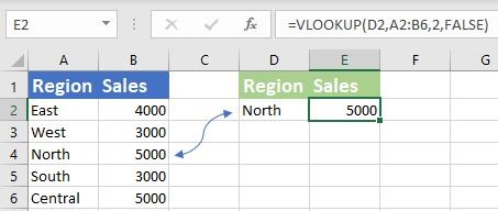
Syntax: =VLOOKUP(lookup_value, Range, 2, FALSE)

Example: =VLOOKUP(“North”, Range(“A2:B6”, 2, FALSE)

‘OR =VLOOKUP(D2, Range(“A2:B6″, 2, FALSE)

This will find the Region”North” in Column A (A2:A6) and return the corresponding value in the Column B (B2:B6). It will return #NA if it finds no match.

2. VLookUp Syntax to Return Approximate Match:

Following is the Syntax and Example to search for a value in the target array and return the corresponding value in the 2nd column.

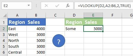
Syntax: =VLOOKUP(lookup_value, Range, 2, TRUE)

Example: =VLOOKUP(“Some”, Range(“A2:B6”, 2, FALSE)

This will search for the given Region name in column A (A2:A6) and return the corresponding value in the Column B (B2:B6). It will return approximate search result if it finds no match.

Purpose

VLOOKUP Function is one of the most using and powerful formulas in the Excel. Often, we search for a value in a array of values and find the corresponding value for further process. For example, we can find Sales of a given Department. We can search for a name in the huge directory and list the respective column values in a range.

Search for a String and Return the Column Value
Check if a Value exist in a Row or Column
Return the information from Table Fields of a matching record
Find a value in an Array of Values and Return respective data from multi dimensional Array

VLOOKUP Usage Steps & Instructions

Many Excel Users wants to understand How to Use VlookUp? Here are the Simple instructions and Examples to explain the usage of VLOOKUP Function in nutshell. We can specify the lookup value, lookup range, lookup column and match type to return the matched values.

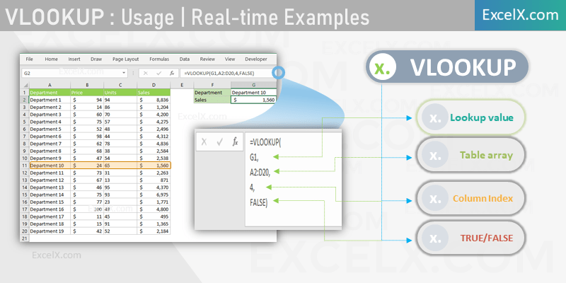
First Argument: Specify the Lookup value to Search for in the left most column of the given range, table or array. Example: G1
Second Argument: Enter the Range, Reference, Named Range, Table or any Array as table_array to look for the first argument (lookup_value). Example: A2:D20
Third Argument: Column Number from the Left side of the Table Array (Second Argument) which you wants Excel to pick and return the corresponding value of the matched record. Example: 4
Fourth Argument: TRUE or FALSE to tell the Excel to perform Approximate or Exact Match. In most cases, it is FALSE (We want to return the column value of the Exact Match). Example: FALSE. DO NOT omit this argument if you want to perform Exact Match, as the default value is TRUE (Approximate Match)

Here is the Example File, VlookUp function is explained with Syntax, Examples and Uses with Simple Step by Step Instructions.

Return Values

VLOOKUP Function return the Following Values when you pass the arguments to the Function.

Returns the columns value of the Exact Match when it find the lookup_value
It will return the #NA when the lookup_value is not found in the left most column of the table_array
If you pass the last parameter as TRUE, it will return the nearest value when it is not found the exact match

Best Practices

Here are the best practices to be followed while using Excel Vlookup Function.

Match type: Most Cases we search for Exact Match and return its correspond=ding Value. Please Make sure to set the fourth Parameters to FALSE (or 0) for Exact Match.
Reference Type: We refer Cells, Rows, Columns, Ranges, Sheets, Workbooks, Named Ranges, Tables, Table Fields while creating VLookUp Formula. Make sure that you are using right type reference (Relative and Absolute Cell References)
Error Handling: VLOOKUP troughs #NA Error if lookup values is not in the first column of the table array data. We can use the Functions IFERROR, IFNA, ISNA Function can help to handle if the return value is an error data type.

Points to Remember:

Please remember and note the following Points while using Excel Vlookup Formula. Understanding the below points will help you to avoid Issue and troubleshooting the Formula.

VLOOKUP is Case sensitive
It looks from left to right
Returns the first matched instance
Can not handle multiple Criteria. Alternatively, use Index, Match functions and create Array formula

Formulas

Examples

VLOOKUP Formula with Example

Download Example Files

Related Functions:

In most scenarios, we use VLookUp function with the following Excel formulas

XLOOKUP: Latest and dynamic Excel Builtin Formula to Lookup the Values in any direction.
HLOOKUP: HLookUp Performs the Horizontal lookup in excel. It will search for a lookup value in the first row of the table and returns the corresponding value of the specified Row in the target range.
IFERROR: We can handle the #NA Error using IfError and VLOOKUP
IF: If Function helps to check if the return value is matching with required value and take the decision.
MATCH : MATCH Function in Excel used to find the match position of a lookup value in a Range, Table and Array.
INDEX : Excel INDEX returns the value of a given position of a Range, Column, Row, Table and Array.

We create Advanced VLOOKUP Formulas by using MATCH and INDEX functions together .

VLOOKUP Function in Excel